Data Driven Money

Live. Work. Retire. Smart.

Simulate Dollar Cost Averaging with Python

Dollar Cost Averaging is the process by which an investor enters an investment position over a series of installments. Generally, either a lump sum is spread out over a predetermined amount of time or a commitment to invest is made using one’s income.

Dollar Cost Averaging

Either way, the affect of Dollar Cost Averaging into an investment is that the volatility of the entry price is reduced… some of the purchases will be at a high price, some will be low. But over the long term the price is an average of all the entry points.

If you are Dollar Cost Averaging because you are earning the investment money while working, then alternative methods of investing may not even be available. Regardless, it would be beneficial to have some ability to simulate how this investing style may compound one’s capital over time.

In this article, I will give you the Python code necessary to simulate a Dollar Cost Averaging (DCA) investment using any type of security you would like. Additionally, I will show you how to plot out your performance against other metrics (again, this may not necessarily be an alternative for many).

In this Article

Getting Started

If you are new to Python then I suggest using Google Colab to execute your code. All the necessary Python dependencies are already installed in a virtual instance that can be accessed via a web browser. Best of all, the service is free. I wrote a very short article on how to get started with Google Colab in case you need a little extra help.

When using Colab, sometimes you will need to install the packages. For this article, the only package that would need to be installed is yfinance which we will use to obtain financial pricing data.

From there, we will need to load the necessary libraries and tweak a quick pandas option to make viewing doubles a bit less obtuse… variables of type float will have numbers only displayed to 2 decimals.

				
					!pip install yfinance

# libraries for working with our data
import pandas as pd
import numpy as np
import yfinance as yf
import datetime

# libraries for plotting
from matplotlib import pyplot as plt
import seaborn as sns

# Use Pandas to reformat columns to be displayed as currency
pd.options.display.float_format = '{:6.2f}'.format


Downloading Stock Pricing Data

Next we are going to need to download the data of our selected investment. This may be a mutual fund, index fund or individual security. Yahoo! Finance offers a wide range of data through its API which can be subsequently accessed using the yfinance package that we loaded previously.

In the code below I have set the options to allow me to download 5 years’ worth of pricing data on the S&P Index fund with ticker symbol ‘SPY.’

The maximum interval for this package is 1 day but when we actually start working with the data we will focus on Dollar Cost Averaging on a monthly basis.

				
					# first, we need to get a hold of the appropriate data
# so we can eventually simulate our dollar cost average method
data = yf.download( 
    
        # download only the tickers we want
        # In this example I will use 'SPY' which
        # attempts to track the performance of the S&P 500
        tickers = "SPY",

        # What period of time are we interested in?
        # valid periods: 1d,5d,1mo,3mo,6mo,1y,2y,5y,10y,ytd,max
        # In our case we will choose 10y
        period = "5y",

        # Next we need to define our interval.
        interval = "1d",

        # Ensure our data is grouped properly.
        group_by = 'ticker',
)

# take a peek at our data
data.head()


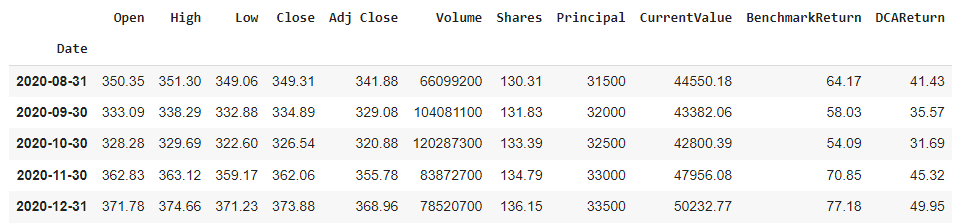
Below is a screen shot of the resulting DataFrame returned by yfinance. The date is set as the index. The column we will be most interested in is the ‘Adj Close’ field… not ‘close.’ The adjusted close considers dividends and any type of stock splits that may distort the pricing data over time.

By using this field, we will also be assuming that any dividends earned will be reinvested. This is an important distinction in that dividends can return several hundred basis points a year. When compounded they can drastically impact the final balance.

yFinance Resulting DataFrame

Dollar Cost Averaging Parameters

Next, we need to define the parameters of our Dollar Cost Averaging exercise. Much like the Compound Interest Calculator I created in Python, we need to establish the starting principal and the reoccurring monthly contribution. Those variables are set below.

Additionally, the starting and ending month and years are set. The reason I decided to use integers instead of a date typed variable is to make the code as accessible as possible. There are certainly shorter and more elegant ways to conduct some of this, however the goal here is to make the code completely accessible to beginners.

				
					# now we need to define the parameters of our dollar cost average

# the starting principal
p = 10000

# the amount to dollar cost average per month
monthly_add = 500

# starting date
starting_year = 2017
starting_month = 1

# ending date
ending_year = 2021
ending_month = 12


Calculating Contribution Dates

Based on the starting and ending timeframes, it is now useful to calculate a Series composed of all the dates that the additional contributions will be transferred on. For our purposes here, I have chosen to select the last day of each month. Likely, most folks decide to contribute after they have made a month’s work. This could look like an automatic withdrawal or even a 401k deposit.

				
					# calculate the number of periods (number of months for the excercise)
periods = (ending_year - starting_year - 1) * 12 + (ending_month - starting_month + 1)

# create a date variable based on starting year and month above
starting_date = str(starting_year)+'-'+str(starting_month)+'-01'

# use starting_date and number of periods (months) to create a series of all 
# contribution dates
contribution_dates = pd.Series(pd.date_range(str(starting_date), freq="M", periods=periods))
contribution_dates.head()


After I calculate the dates, I then store them in a variable called contribution_dates. The output of the first few entries can be seen below.

Contribution Dates Output

Removing Weekends and Non-Trading Days

Just contributing your DCA amount at the end of each month sounds simple enough, however, for computational purposes its too simple. The last day of a month may include a weekend, a holiday, or some other non-trading day for which the data set we downloaded will be insufficient.

To account for this I have created a very simple and blunt force approach. If a day in contribution_dates cannot be found in the set of dates downloaded into to data then that date is moved 1 day earlier. If the date is a Sunday then it will be moved to the previous Saturday. This done iteratively until the date matches a trading day within data.

As you will see, I only had to run through this algorithm twice. You may find that given the dates you select and the security chosen you may have to iterate further.

				
					# quickly print out all contribution dates that were not trading days
for i in range(len(contribution_dates)):
  if contribution_dates[i] not in data.index:
    print(contribution_dates[i], contribution_dates[i].day_name())


Contribution Dates not Trading Dates Output

				
					# If the day is not a trading day then move it one day previous and store
for i in range(len(contribution_dates)):
  if contribution_dates[i] not in data.index:
    contribution_dates[i] = contribution_dates[i] - pd.Timedelta("1 day")

# Once again print out the dates to see how we did
for i in range(len(contribution_dates)):
  if contribution_dates[i] not in data.index:
    print(contribution_dates[i], contribution_dates[i].day_name())


Contribution Dates not Trading Dates 2

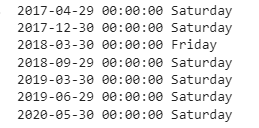
After one round of moving dates to the left the number of records that were not actually trading days drops from 13 down to 7.

				
					# Iterate one more time though the list to move dates to the left
for i in range(len(contribution_dates)):
  if contribution_dates[i] not in data.index:
    contribution_dates[i] = contribution_dates[i] - pd.Timedelta("1 day")

# Print all the results out that are not trading days. Hopefully, 
# the printout will be NULL
for i in range(len(contribution_dates)):
  if contribution_dates[i] not in data.index:
    print(contribution_dates[i], contribution_dates[i].day_name())


Thankfully, the second printout is in fact NULL. All dates in contribution_dates are now guaranteed to have a matching record in data.

Creating a DataFrame with our Results for DCA

Next, it’s finally time to calculate the results of dollar cost averaging over time. I have decided to do this with a for loop. Again, this may be a tad inefficient, but it makes the calculations easily understandable (and customizable) by those who may spend more time working in the financial advisory field than the python programming world.

The loop is used to calculate 5 different things. The result for each item is then stored in the data DataFrame for each period. The calculations are iterative, so each successive calculation requires the previous month to have been calculated first. The columns of data created are the following:

  • Shares – The current number of shares of the security owned. This includes the current month’s contribution.

  • Principal – This keeps track of how much principal (no investment growth) has been used to purchase the security over time.

  • CurrentValue –This field uses the Share count and final adjusted price for the month to determine the current market value at that time.

  • BenchmarkReturn – This keeps tabs on how much the security has gone up in terms of percentage points since the beginning of the overall time period up to that point. This number is not averaged or annualized. It’s just the raw return over the entire time period.

  • DCAReturn – This is the amount of return based on the running total. This is not adjusted for each month, rather it gives a total snapshot of how much has been returned. There are other ways to calculate this metric so be careful!
				
					# Establish new columns with our starting principal, number of shares
# Current Value of our shares, the running return of the selected security
# and the Dollar Cost Averaging Running Return
data['Shares'] = p / data.loc[contribution_dates.iloc[0], 'Adj Close']
data['Principal'] = p 
data['CurrentValue'] = p
data['BenchmarkReturn'] = 0
data['DCAReturn'] = 0

for i in range(1, len(data.loc[contribution_dates])):
  # Calculate the number of Shares added by the contribution and add to previous month's amount
  data.loc[contribution_dates.iloc[i], 'Shares']  = data.loc[contribution_dates.iloc[i-1], 'Shares'] + (monthly_add / data.loc[contribution_dates.iloc[i], 'Adj Close'])
  
  # Add the monthly contribution at the beginning of each month to the principal
  data.loc[contribution_dates.iloc[i], 'Principal']  = data.loc[contribution_dates.iloc[i-1], 'Principal'] + monthly_add
  
  # Use the present value of the security to find the total value of all shares owned
  data.loc[contribution_dates.iloc[i], 'CurrentValue']  = data.loc[contribution_dates.iloc[i], 'Shares'] * data.loc[contribution_dates.iloc[i], 'Adj Close']
  
  # Calculate the running return of the security based on the current month's price (iterative)
  data.loc[contribution_dates.iloc[i], 'BenchmarkReturn'] = (data.loc[contribution_dates.iloc[i], 'Adj Close'] - data.loc[contribution_dates.iloc[0], 'Adj Close'])/data.loc[contribution_dates.iloc[0], 'Adj Close']*100
  
  # Calculate the running return of the DCA balance on the current month's price (iterative)
  data.loc[contribution_dates.iloc[i], 'DCAReturn'] = (data.loc[contribution_dates.iloc[i], 'CurrentValue'] - data.loc[contribution_dates.iloc[i], 'Principal'])/data.loc[contribution_dates.iloc[i], 'Principal']*100

# Create a new DataFrame that only has rows corresponding to the contribution dates
monthly_data = data.loc[contribution_dates]

# Print out the last 5 months worth of results
monthly_data.tail()


Dollar Cost Averaging Calculated

Plotting Dollar Cost Averaging Results with Python

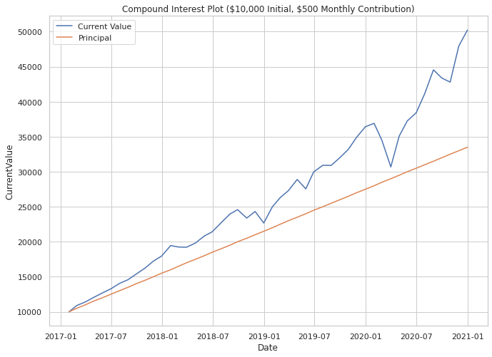
Using the MatPlotLib and Seaborn libraries it is now easy to create a couple of plots that can help us interpret how our DCA simulation performed. In the plot below, I simply plotted the CurrentValue and Principal fields across all contribution dates.

The resulting plot gives a clear depiction of how the returns in SPY helped our fictional investor compound their earnings over time. The disparity between the orange and blue lines gets larger and larger over successive periods. It should be noted that the during the time periods used, the S&P 500 went mostly up… but so does the Stock Market in general over long periods.

If the SPY had been declining over the entire period, we should subsequently expect to have not performed better against the principal.

				
					# Now Let's go ahead and plot it out
sns.set(rc={'figure.figsize':(11,8)}) # Change the size of the plot
sns.set_style('whitegrid') # Change the default background
plt.ticklabel_format(style='plain', axis = 'y') # prevent sci notation on y-axis

# now for the actual plot
sns.lineplot(data = plot_data, x= 'Date', y = 'CurrentValue')
sns.lineplot(data = plot_data, x= 'Date', y = 'Principal').set_title('Compound Interest Plot (\$10,000 Initial, \$500 Monthly Contribution)')
plt.legend(labels=["Current Value","Principal"])


Compound Interest Plot from Dollar Cost Averaging with SPY

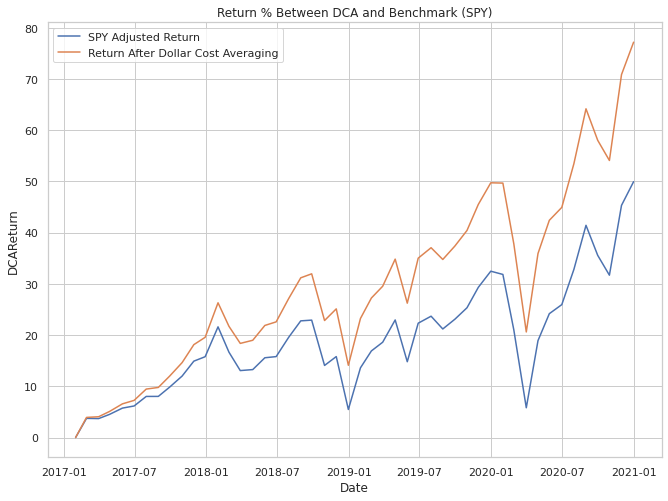
Comparing Dollar Cost Averaging and the Benchmark

Another interesting plot can be used to verify that what we think has been calculated actually makes sense. Dollar Cost Averaging will result in a higher cost basis over time if the underlying asset is increasing over the entire period. As each successive month rolls on buy, the purchase price of the stock or security goes up.

Given this, if the underlying benchmark is going up in price we should expect our plotted line for our investment to be below that line. This does not mean that DCA has failed, it only helps us verify that what we calculated is in fact what we were expecting.

On the other hand, if you had started investing at a market peak and successively purchased in for a period of time where the price declined you could expect that your performance on a percentage terms outperforms the market. Take a gander below at a comparison of performances based on % terms of the data we have been using:

				
					# now for the actual plot
sns.lineplot(data = plot_data, x= 'Date', y = 'DCAReturn')
sns.lineplot(data = plot_data, x= 'Date', y = 'BenchmarkReturn').set_title('Return % Between DCA and Benchmark (SPY)')
plt.legend(labels=["SPY Adjusted Return","Return After Dollar Cost Averaging"])


Return Percentage Between DCA and the SPY

Summary

In this article I have showed you how to pull in market data for a stock through Yahoo! Finance using python and then simulate how an investment may perform if you utilized Dollar Cost Averaging. Understanding the potential compound growth opportunities in the market can help not only educate but also motivate potential investors.

Additionally, understanding how investment performance differs when using DCA vs a lump sum investment during market extremes may also help those that have suddenly come upon a large windfall of money.

I hope you enjoyed this article! I love getting feedback both positive and constructive so head to the comments section if you have anything you would like to share!

Guy Money

As a formally trained Data Scientist I find excitement in writing about Personal Finance and how to view it through a lens filtered by data. I am excited about helping others build financial moats while at the same time helping to make the world a more livable and friendly place.

Leave a Reply

Your email address will not be published. Required fields are marked *

Scroll to top