Data Driven Money

Live. Work. Retire. Smart.

How to Use Python to Model Paying Off Your Mortgage Early

Home Amortization with PythonPurchasing a home is one of the biggest decisions an individual can make over the course of their entire lifetimes. Developing the credit history and income to convince a bank to fork over multiple times your annual salary is quite the feat. However, paying off your mortgage can often be just as big a of a decision.

In this article I will show you how to wield Python to calculate the benefit of paying additional money towards your mortgage. Scenarios where an additional amount is paid every month, or even midway through the loan period will be considered.

Finally, I will show you how to plot this information out using the MatPlotLib and Seaborn libraries.

Graphically depicting the benefit of paying additional money towards your home loan can be quite motivational and a helpful explanatory tool when describing these benefits to others such as your spouse or even perhaps clients.

How We'll Tackle Paying Additional Payments in Python

Getting Started

To compile and run my code I have decided to use Google Colab

Colab is a web-based python environment that allows you to use a Jupyter like notebook via a web browser since the backend is in the cloud. This makes configuring and managing the underlying environment trivial. You can use Google Colab for free at this link to follow along with the code provided.

Below is the code necessary to import the appropriate libraries.

Pandas and Numpy are used for simple data manipulation. MatPlotLib and Seaborn are used for displaying plots. The final line of code is used to massage the output of float typed variables… we set this to make the output look like dollars and cents with only 2 decimal points used for precision.

				
					# Import the appropriate libraries
import pandas as pd
import numpy as np

# These libraries will be used later to plot our data
from matplotlib import pyplot as plt
import seaborn as sns

# Use Pandas to reformat columns to be displayed with only
# two decimal points... like a currency
pd.options.display.float_format = '{:6.2f}'.format


Codifying the Mortgage’s Specific Parameters

To calculate an early payoff to a mortgage, the defining characteristics need to be input as variables. The three pieces of information required are:

  • The principal or starting loan amount (P)
  • The interest rate of the loan (r)
  • The number of months of the entire loan from start to finish (n)

Below, these parameters are set. For this article, a home with a starting principal of $100,000 at a rate of 6% interest with a loan period of 30 years (360 months) is used.

				
					# Establish Initial Parameters in order to Amoritize the original loan

# P is the principal amount of the original loan
P = 100000

# r is the rate of interest per expressed as a decimal
r = 0.06

# n is the number of periods (months)
n = 360


Amortizing the Mortgage

In another article I wrote, I showed how to use Python to Calculate Mortgage Amortization. The formula is fairly straightforward. To calculate the Total Monthly Payment for a Mortgage given the parameters set above you would use this formula:

Mortgage Amortization Formula

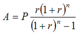
Note: This formula should be used with the monthly interest rate for r. Our parameters set above use the more traditional annual interest rate. I will convert r to rM below which will account for this.

				
					# rM is derived from r. It is the monthly interest rate
rM = r/12

# A is the monthly payment amount. A is derived from the above paremeters
A = P * (rM*np.power((1+rM), n))/(np.power((1+rM),n)-1)

# Display our Monthly Payment
print(round(A,2))


The variable A above is the Total Payment as expected. When printed, the result is $599.55.

Since this is the Total Payment, it is composed of both a portion that will pay down the principal and a portion that will be used to pay the month’s interest to the lender.

Moving forward, we will want to know specifically how each monthly payment breaks down. Over time the amount going towards the principal will increase and the amount going towards interest will decrease. This is all despite the Total Payment remaining fixed.

Below is the code necessary to calculate these parameters and output the results to the console for the first month only.

				
					# Now that we know the total payment we now need to figure
# out the breakdown between principal and interest being made

# For the first month we just mulitply the principal my the monthly
# interest rate to determine how much was paid in interest during
# the first month
I = P * rM

# Print out some stats
print("The Total Monthly Payment in month 1 is: ", round(A,2))
print("Total Interest Paid as a Component is:   ", I)
# Thus,  A - I = the amount of principal paid during the first month
print("Total Interest Paid as a Component is:   ", round((A - I), 2))


Output of Mortgage Amortization Breakdown

Finding the Payment Breakdown for All Months

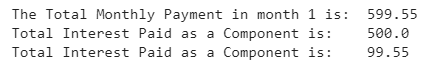
Calculating the 1st month’s breakdown was simple. However, we now need to find the breakdown of interest and principal for each month of the entire loan.

Using a for loop I will populate a DataFrame called data. data will be initialized with the first month’s data at the outset. The principal paid in the first month will be subtracted from the overall principal remaining on the loan so that the next month’s interest can be calculated.

From there the process repeats until all months have been addressed and the final payment covers the entire remaining principal and accrued interest.

				
					# Now let's find out the breakdown of interest and principal for each period.
# I'll store the interest, principal and total payment for each month in a row
# of a DataFrame by iterating through with the above information. 

data = pd.DataFrame(columns = ['Month','TotalPayment','Interest','Principal'])

# Intializng variable for the loop for Month 1 as previously calculated


# Append Month 1 data to data
Month = 1
TotalPrincipal = P
TotalPayment= A
Interest = I
Principal = A - I

data =  data.append({'Month': Month,
                     'TotalPrincipal': TotalPrincipal, 
                     'TotalPayment': TotalPayment,
                     'Interest': Interest,
                     'Principal': Principal}, ignore_index = True)

for j in range(1, n):
  # Compute the 
  # Recompute the Payment Information
  Month = j+1
  TotalPrincipal = data.loc[j-1]['TotalPrincipal']- data.loc[j-1]['Principal']
  TotalPayment = TotalPayment
  Interest = TotalPrincipal * rM
  Principal = TotalPayment - Interest
  
  # append Month J's Payment Information
  data =  data.append({'Month': Month,
                       'TotalPrincipal' : TotalPrincipal,
                       'TotalPayment': TotalPayment,
                       'Interest': Interest,
                       'Principal':Principal}, ignore_index = True)

# Fix the Month to be an integer
data['Month'] = data['Month'].astype(int)

# Now let's take a look at every Month's payment and breakdown
data


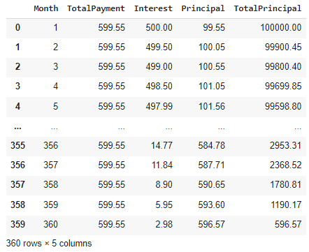
Taking a peek below at data reveals that there is a row for each month. The index runs from 0 to 359 and the final payment (row 359) is composed of the exact amount necessary to complete the terms of the mortgage.

Output of Data Calculated for Each Month of Mortgage

Paying Additional: Calculating the Data

Now that we know how the original loan is amortized and how to calculate the breakdown of the interest and principal components for each payment it is time to add in our additional monthly payment.

Below, the variable AdditionalPayment can be changed to account for whatever amount you would like to pay extra. I have set AdditionalPayment to $300. For this portion, the additional amount will be applied for all payments of the loan… even the first payment (we will cover more complicated scenarios later).

The setup for this calculation is almost exactly the same as for the original amortization. The resulting DataFrame will be called data_addpay.

				
					# Additional Monthly Amount

# I will use the same method as above but add an additional variable called
# 'AdditionalPayment' which I will initialize as $300

data_addpay = pd.DataFrame(columns = ['Month',
                                      'TotalPayment',
                                      'Interest',
                                      'Principal',
                                      'AdditionalPayment'])

Month = 1
TotalPrincipal = P
TotalPayment= A
Interest = I
Principal = A - I
AdditionalPayment = 300

data_addpay =  data_addpay.append({'Month': Month,
                                   'TotalPrincipal': TotalPrincipal, 
                                   'TotalPayment': TotalPayment,
                                   'Interest': Interest,
                                   'Principal': Principal,
                                   'AdditionalPayment': AdditionalPayment},
                                   ignore_index = True)

for j in range(1, n):
  Month = j+1
  # Below is where I subtract an the Additional Amount
  TotalPrincipal = data_addpay.loc[j-1]['TotalPrincipal'] - data_addpay.loc[j-1]['Principal']-AdditionalPayment 
                 
  TotalPayment = TotalPayment
  Interest = TotalPrincipal * rM
  Principal = TotalPayment - Interest
  
  # append Month J's Payment Information
  data_addpay =  data_addpay.append({'Month': Month,
                                     'TotalPrincipal' : TotalPrincipal,
                                     'TotalPayment': TotalPayment,
                                     'Interest': Interest,
                                     'Principal':Principal,
                                     'AdditionalPayment': AdditionalPayment},
                                     ignore_index = True)


The output of data_addpay can be seen below.

Output of Data Calculated for Each Month of Mortgage with Added Amount

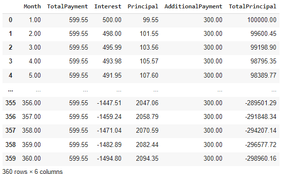
Notice that the number of Months in the final row is still 360. But does this make sense? It looks like the calculation just continued even after the loan was paid.

There are 2 main ways to tackle this:

  • We could add an if statement into the for loop to escape earlier based on the value of
  • We can just truncate the data that we have already calculated.

I will opt for the latter as seen below. The first step is to find PayOffMonths, or the number of months that will be used to truncate the data.

				
					# Fix the Month to be an integer
data_addpay['Month'] = data_addpay['Month'].astype(int)

# Using this method we will need to find where in this new and expectedly shorter
# DataFrame the TotalPrincipal has turned negative. This implies that the Home
# Mortgage has been fully paid off during this month

# Narrowing our results to just months with negative amount, then filtering down
# to just the first record's value of 'Month'
PayOffMonths = np.int(data_addpay.loc[data_addpay['TotalPrincipal']<=0].iloc[0]['Month'])-1
PayOffMonths


The result for our scenario for PayOffMonths is 163. After 163 months, vice 360, our loan will be paid off if $300 is paid on top of the normal payment each and every month.

Thus, in order to truncate data_addpay I will do the following:

				
					# Truncating our DataFrame to only relevant months
data_addpay = data_addpay.loc[data_addpay['Month']<= (PayOffMonths)]
data_addpay


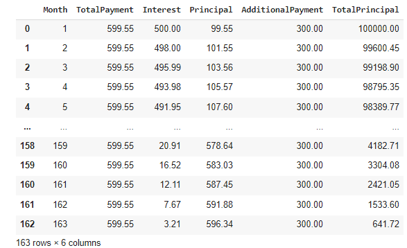
And the new version of data_addpay can be seen below to have only 163 rows as expected. We now have all the data necessary to make a quantitative comparison… and even make a plot!

Output of Data Calculated for Each Month of Mortgage with Added Amount Fixed

Paying Additional:  Plotting a Comparison to the Original Mortgage

With the data of both the original amortization and of the scenario where an additional payment of $300 is added on top of each month’s payment we can quickly plot how they compare.

				
					# Plotting Payoff Scenario Comparison

sns.set(rc={'figure.figsize':(11,8)}) # make the graph readably large
sns.set_style('whitegrid') # change the background grid
sns.set_palette('Greens') # hange the color scheme

sns.set(font_scale = 1.75) # make titles and axis names larger

# Plotting interest and principal components as a scatterlot
addpay_plot = sns.scatterplot(data = data_addpay, x ='Month', y = 'TotalPrincipal', color = 'red')


orig_plot = sns.scatterplot(data = data, x ='Month', y = 'TotalPrincipal', color = 'blue').set_title('Original Payment Vs. Additional Payment')
print("Payoff Months: ", PayOffMonths)


We should expect two sloping lines. The original loan data will slope towards 0 after 360 months. The additional payment data should slope much more steeply and terminate at month 163.

Plot Comparing Amortizations of Original and Additional Payment

As seen above, the plot appears as expected. We can clearly see the effect of paying additional. But what if we only start paying an additional amount starting at some point after month 1? This is likely the most useful consideration. We’ll cover this tweak in the next section.

Paying Additional: Custom Start Date for Additional Payments

As a mortgage borrower, likely the decision to pay additional towards the principal will come at least a few months after you have started making payments. Perhaps it will be years. Whatever the case, it is easy to modify the code we have already wrote to account for this.

The initial data needed is below. The variable MonthStartContributing will be number of the montsh into the original loan period that the borrower intends to start adding an additional payment to be paid towards the principal.

				
					# Additional Monthly Amount Starting at a Certain Month
MonthStartContributing = 120

# Additional Monthly Amount with Custom Month Calculation
# To do this I will just start with the original amoritization method
# then modify the additional contribution amount in a second loop
data_custom = pd.DataFrame(columns = ['Month',
                                      'TotalPayment',
                                      'Interest',
                                      'Principal',
                                      'AdditionalPayment'])

Month = 0
TotalPrincipal = P
TotalPayment= A
Interest = I
Principal = A - I
AdditionalPayment = 300

data_custom =  data_custom.append({'Month': Month,
                                   'TotalPrincipal': TotalPrincipal, 
                                   'TotalPayment': TotalPayment,
                                   'Interest': Interest,
                                   'Principal': Principal,
                                   'AdditionalPayment': AdditionalPayment},
                                   ignore_index = True)  


In the code below I will combine the two for loops used for the original loan amortization and the one for additional payments from above. The first loop stops at the month prior to the one selected for making additional payments.

				
					for j in range(1, MonthStartContributing-1):
      Month = j+1
      # Below is where I subtract an the Additional Amount
      TotalPrincipal = data_custom.loc[j-1]['TotalPrincipal'] - data_custom.loc[j-1]['Principal']
                 
      TotalPayment = TotalPayment
      Interest = TotalPrincipal * rM
      Principal = TotalPayment - Interest
  
      # append Month J's Payment Information
      data_custom =  data_custom.append({'Month': Month,
                                         'TotalPrincipal' : TotalPrincipal,
                                         'TotalPayment': TotalPayment,
                                         'Interest': Interest,
                                         'Principal':Principal,
                                         'AdditionalPayment': AdditionalPayment},
                                         ignore_index = True)


The second loop picks up where the other one left off and runs for the full number of periods n (in this case, 360 months).

				
					for j in range(MonthStartContributing-1, n):
  Month = j+1
  # Below is where I subtract an the Additional Amount
  TotalPrincipal = data_custom.loc[j-1]['TotalPrincipal'] - data_custom.loc[j-1]['Principal']-AdditionalPayment 
                 
  TotalPayment = TotalPayment
  Interest = TotalPrincipal * rM
  Principal = TotalPayment - Interest
  
  # append Month J's Payment Information
  data_custom =  data_custom.append({'Month': Month,
                                     'TotalPrincipal' : TotalPrincipal,
                                     'TotalPayment': TotalPayment,
                                     'Interest': Interest,
                                     'Principal':Principal,
                                     'AdditionalPayment': AdditionalPayment},
                                     ignore_index = True)

# Fix the Month to be an integer
data_custom['Month'] = data_custom['Month'].astype(int)


From there, just like before, the data is truncated to only include the relevant months where the TotalPrincipal is above 0. The data is stored in data_custom and can be seen below.

				
					PayOffMonths = np.int(data_custom.loc[data_custom['TotalPrincipal']<=0].iloc[0]['Month'])-1

# Truncating our DataFrame to only relevant months
data_custom = data_custom.loc[data_custom['Month']<= (PayOffMonths)]
data_custom


As can be seen above, it takes 245 months in this scenario to pay off the loan.

Full Analysis: Originally, it required 360 months to pay off $100,000 at 6% interest. With $300 added each month it took 163 months. However, if $300 is only added after 10 years (120 months) of repayment have occurred then it will take 245 months to completely pay off the loan.

Paying Additional: Plotting a Comparison to the Original Mortgage Part 2

When plotting this chart, we should expect to see the original blue line descending to 0 over the course of 360 months like before. Nothing has changed about the original mortgage amortization.

What will be different is the second line should appear to branch off the original line at the month that the additional payments are made. The second line should clearly show that the balance reaches 0 much earlier.

Below is the code and resulting plot it generates once executed

				
					# Plotting Modified Payoff & Custom Payoff Scenario Comparison

# Plotting interest and principal components as a scatterlot
custom_plot = sns.scatterplot(data = data_custom, x ='Month', y = 'TotalPrincipal', color = 'green')
orig_plot = sns.scatterplot(data = data, x ='Month', y = 'TotalPrincipal', color = 'blue')\
                        .set_title('Original Vs. Additional Mortagage Payment Starting at Specific Month')
                        
print("Payoff Months: ", PayOffMonths)


Plot Comparing Amortizations of Original and Additional Floating Payment

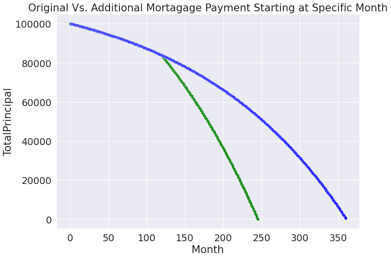
The plot matches our original expectations.

Paying Additional: Plotting a Comparison to the Original Mortgage Part 3

Now let’s plot all 3 together. The code in this case is very much just a copy and paste of the above.

				
					# Plotting Custom Payoff Scenario Comparison

# Plotting interest and principal components as a scatterlot
custom_plot = sns.scatterplot(data = data_custom, x ='Month', y = 'TotalPrincipal', color = 'green')
orig_plot = sns.scatterplot(data = data, x ='Month', y = 'TotalPrincipal', color = 'blue').set_title('All Three Payment Methods')
addpay_plot = sns.scatterplot(data = data_addpay, x ='Month', y = 'TotalPrincipal', color = 'red')


Plot Comparing Amortizations of all 3 Scenarios

With this final plot is easy to confirm all our theories with the data that was calculated. Additionally, the code we have created is in perfect form to create our own function in Python which I will do in another article.

More complicated analytical investigations can be completed that vary both the additional payment used, interest rate, and other technical aspects of the mortgage with this work used as a basis.

Summary

In this article I have showed you how to calculate the amortization of your mortgage, apply an additional payment throughout the loan, and apply an additional payment partially through the loan. I have shown you how to plot the resulting data and think about how to evaluate the results to ensure their validity.

I hope you enjoyed this article! I will be adding more complicated scenarios as a follow-up and will post them here at DataDrivenMoney.com as always. Please feel free to throw positive or constructive comments in the section down below!

Guy Money

As a formally trained Data Scientist I find excitement in writing about Personal Finance and how to view it through a lens filtered by data. I am excited about helping others build financial moats while at the same time helping to make the world a more livable and friendly place.

Leave a Reply

Your email address will not be published. Required fields are marked *

Scroll to top