Data Driven Money

Live. Work. Retire. Smart.

Calculate the Stock Market CAGR with Python

The Compound Annual Growth Rate (CAGR) is a superior metric that is often overlooked when trying to understand the performance of various stocks. Using Python, the calculation is simple and quick. Additionally, the ability to use real time data further increases the advantages… and all is possible with only a few lines of code.

Calculate Stock Market CAGR with Python

In this article I’ll cover how to pull accurate and timely market data for just about any stock ticker you can think of using the yfinance package available from PyPi. From there I will help you implement the formula for CAGR to quickly compare the performances of multiple stock tickers.

If you aren’t sure on which stock or index to choose then knowing the CAGR, a measure of past performance, may be something that you are interested in.

Table of Contents

What is CAGR and Why Should I Use it?

CAGR is a way of measuring performance by ignoring volatility. I wrote an entire article about the CAGR formula and the nuances of its competitor, the Average Annual Return (AAR). The best way to explain CAGR is by explaining an example using AAR.

With AAR, as its name implies, you just average the annual returns. Take an example portfolio that starts at $100. After the first year it makes 100%, and thus has a value of $200. After the second year it takes a 50% loss… it now finishes the 2 year period at $100. Exactly where it began.

With AAR, the measure of performance would be 25%. That would be the average return over the two years. If I told you that you averaged a 25% return over any period you’d probably be happy… but in this example it resulted in no gain. That’s the flaw of using AAR.

Using CAGR, the following formula would apply:

CAGR Formula

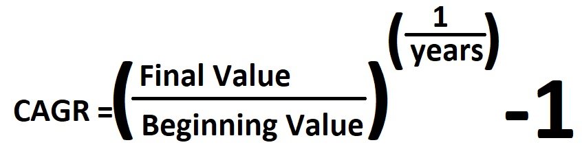
Using this formula, the CAGR for our example would be 0%.  This is exactly what we would have rationally expect. Thus, using CAGR as a measure of performance is a great we to compare equities.

Getting Started in Python

Whether you are a beginner at coding in general, or a veteran, using Google Colab to run these quick Python examples is an easy way to test things out. I have a written a quick and short primer on how to get started with Google Colab here.

By using Google Colab, you will be able to run your code in the cloud for free. All you will need is Chrome. Additionally, many of the Python dependencies that can cause headaches for newbies are solved in advance. Just type a few lines of code and execute. 

Alternatively, you can  use your own Python environment. I personally use Anaconda to help manage my environment but there are an infinite ways to get started. For this article I will be using only a few packages that are readily available on PyPi.

Loading the Necessary Python Packages

The first block of code I wrote is just simply to load the packages. Only 2 packages are used in this short example: numpy and yfinance. numpy is used for the execution of the formula (the power function). yfinance is used to pull the actual stock data into a DataFrame.

				
					# install library not available in colab
!pip install yfinance

# import the necessary libraries
import yfinance as yf
import numpy as np


Pulling the Data from Yahoo Finance

Calculating the CAGR of a security requires the actual numbers. The yfinance package gives numerous ways to access the real time market data provided by Yahoo Finance. For this article I will show you two ways.

Below you will see that I have chosen 2 stock tickers to evaluate. TSLA and VTI. I have set the period to 5y thus I will be downloading a full 5 years of data and at a 1 day interval. When looking at the formula for CAGR, I know I only need the beginning value, final value and time in years to make my calculation. Thus the next snippet of code should give me all I need to proceed.

				
					# download the appropriate data
data = yf.download( 
    
        # download only the tickers we want
        # Which is the Vanguard Total Stock Market Index (VTI)
        # and Tesla (TSLA) in order to compare their CAGRs
        tickers = "VTI TSLA",

        # What period of time are we interested in?
        # valid periods: 1d,5d,1mo,3mo,6mo,1y,2y,5y,10y,ytd,max
        # In our case we will choose 5y
        period = "5y",

        # Next we need to define our interval. For our CAGR
        # Calculation we really only need the beginning and ending
        # values so we will choose the maximum interval value
        interval = "1d",

        # Ensure our data is grouped properly.
        group_by = 'ticker',

)


Calculating the CAGR for Comparison

Now that we have used python to download the appropriate pricing data for our 2 equities, all we have to do is plug them into our formula. I do, however, conduct some data manipulation that does need to occur to streamline the processing… getting rid of the NA’s in our situation doesn’t result in a loss of any necessary information.

				
					# We picked a 5 year time period so that will be the value of t
time_period = 5 

# All that matters when calculating CAGR is the beginning and
# final values. Some of the data has NAs... we'll just drop them
# since it won't affect your calculation
VTI = data['VTI'][['Close']].dropna()

# finally, we will need to know the resulting number of data points
# so we can access the propriate record. This value is stored in
# max_index
max_index = len(VTI['Close'])

# Now let's calculate the CAGR for our first Ticker
VTI_CAGR = np.power((VTI['Close'].iloc[max_index -1]/VTI['Close'].iloc[0]), (1/time_period)) - 1
print("VTI CAGR:", VTI_CAGR)

# Repeat the process for our second Ticker
TSLA = data['TSLA'][['Close']].dropna()
max_index = len(TSLA['Close'])

TSLA_CAGR = np.power((TSLA['Close'].iloc[max_index -1]/TSLA['Close'].iloc[0]), (1/time_period)) - 1
print("TSLA CAGR:", TSLA_CAGR)


Below is the output to the above code snippet. As we can see, the CAGR for the VTI, a broad market index, is a hair over 16% for the past 5 years. This respectable performance is blown out of the water by TSLA’s CAGR which is a whopping 97%. I won’t comment further on either’s performance, however using this code you can see how valuable it could be to quickly gauge past performance.

VTI CAGR: 0.16062853588035786 
TSLA CAGR: 0.9736787744617004

Using Specific Dates for Data

In the above example, we were forced to use  one of the canned time periods for our date range. This is probably not the level of fidelity you were hoping for. Below I have shown a way to pull the stock market price based on specific dates.

Since CAGR’s formula does require a value for t you should be careful about what dates you choose. Using dates that are 3 month periods can obviously be easily used since each period would increase by .25 for t (e.g. 21 months would mean t would be 1.75).

Below the data pull, the CAGR values for both VTI and TSLA were calculated in the same way as before.

				
					# download the appropriate data
data = yf.download( 
    
        # download only the tickers we want
        # Which is the Vanguard Total Stock Market Index (VTI)
        # and Tesla (TSLA) in order to compare their CAGRs
        tickers = "VTI TSLA",

        start="2018-01-01", end = "2020-12-31",

        # Next we need to define our interval. For our CAGR
        # Calculation we really only need the beginning and ending
        # values so we will choose the maximum interval value
        interval = "1d",

        # Ensure our data is grouped properly.
        group_by = 'ticker',

)

# set our time period as before... in this case
# it is 3 years
time_period = 3 

# get rid of the NA values
VTI = data['VTI'][['Close']].dropna()
max_index = len(VTI['Close'])

# calculated CAGR for VTI
VTI_CAGR = np.power((VTI['Close'].iloc[max_index -1]/VTI['Close'].iloc[0]), (1/time_period)) - 1
print("VTI CAGR:", VTI_CAGR)

# Rinse and repeat for our second ticker
TSLA = data['TSLA'][['Close']].dropna()
max_index = len(TSLA['Close'])

TSLA_CAGR = np.power((TSLA['Close'].iloc[max_index -1]/TSLA['Close'].iloc[0]), (1/time_period)) - 1
print("TSLA CAGR:", TSLA_CAGR)


The output below shows that once again VTI has performed well, but TSLA has just been incredible. The values for CAGR were quickly and easily calculated making our analysis of performance instantaneous.

[*********************100%***********************] 2 of 2 completed
VTI CAGR: 0.11915508652149587
TSLA CAGR: 1.2130074508622077

Summary

Using Python to pull market data and calculate the Combined Annual Growth Rates for individual securities on the fly is both quick and efficient. It can be used in a larger data acquisition strategy for both simple analysis and further processing with Machine Learning or AI techniques.

I hope you enjoyed this simple article. Although it was geared towards beginners, the ability to pull market data is a necessary skill for pretty much anything in the Data Science field related to investing.

Guy Money

As a formally trained Data Scientist I find excitement in writing about Personal Finance and how to view it through a lens filtered by data. I am excited about helping others build financial moats while at the same time helping to make the world a more livable and friendly place.

Leave a Reply

Your email address will not be published. Required fields are marked *

Scroll to top