Data Driven Money

Live. Work. Retire. Smart.

How to Use Python to Calculate Compound Interest

Facebook
Twitter
LinkedIn
Pinterest
How to Use Python to Calculate Compound Interest

Table of Contents

The Ease and Power of Python for Personal Finance

Over the years I have found using the Python programming language is a powerful tool in mathematics. As a Data Scientist it has become an easy way to quickly bring a concept into production. As someone who is interested in Personal Finance, however, the tools available to manipulate data are often just out of grasp for Financial Planners. This should not stop you from reaching towards Python, however, when trying to develop an interesting and useful analysis of your own Personal Finance endeavors. In this article, we will be looking at how to do the following:

  • Compute Compound Interest using Python
  • Output our Results to Excel
  • Output our Results to a Bar Chart Using matplotlib and Seaborn

This article is geared towards someone who knows a teeny tiny bit about python… but not much more than that. All of this code can be copied and pasted for use in your own scripts or Jupyter Notebooks. Just change up the variables in the designated section and you should be able to easily calculate compound interest as needed for varying time periods.

Getting Started: Jupyter Notebook and Google CoLab

First thing is first: get your Python environment up and running. If you want to take a 2 hour detour and set up your own Anaconda environment then this tutorial will do the trick. If you are looking for something a bit more simplistic then just using Google Colab is probably your best bet. Colab can be opened in a web browser and the actual computation happens in the cloud. Google provides enough CPU resources for free, so this is a no cost venture. Just open a web browser and start coding…

Screenshot of Google Colab

One of the big things that I really like about using Google Colab is that I can run my code anywhere at any time. I can access and run the same code from my phone, at work or at home just in the same way. When I want to run a quick thought experiment, I can type it in real quick and boom… code written, executed, and stored in the cloud for further analysis later.

Writing the Code: Using Python to Calculate Compound Interest

To begin, we will need to import 4 different libraries. We will need pandas and numpy for basic data and numerical manipulation. We will also need matplotlib and seaborn. These two libraries will work together to give us the look and feel we want from the plots we will eventually make. An additional option is set on the last line. This line will ensure that after our computations are made, the results will carry a decimal with only 2 places to the right… just like dollars and cents. Otherwise, scientific notation is the default which makes it difficult to quickly make judgements about the data we’ve created.

				
					# import the appropriate libraries

# need these for data manipulation
import pandas as pd
import numpy as np

# need these for plotting
from matplotlib import pyplot as pyplot
import seaborn as sns

# Format money columns to two decimal places in pandas
pd.options.display.float_format = '{:6.2f}'.format


The next code block is where you will put your specific information. You can set the principal, or the starting amount with the variable ‘p’. ‘r’ is the interest rate for the period. ‘n’ is the number of times the amount should be compounded per period. And ‘t’ is the number of periods. So, for example, if you wanted to see what $10,000 at a rate of 10% over 7 years, compounded at the end of each year comes out then would use the settings you see below. Feel free to tweak this in your own code to the calculation that makes sense for you.

				
					# prepare our variables

###############################################################
###############################################################
## Change the Below Variables for your investment scenario

P = 10000 # our starting principal
r = 0.1 # our interest rate of 10%
n = 1 # the number of times compounded per period
t = 7 # the number of periods

###############################################################
###############################################################


The following code block does the grunt work. It establishes a Pandas DataFrame that will be used to store our results. We will store the Period and Amount for each period. To do this we will use a for loop that will iterate over the number found in the variable ‘t’. The formula for compound interest and what is encoded below is the following:

results = P * (1 + r/n)n * t

When we finish all that, we will ensure that our Period is stored as an integer so that it doesn’t have a decimal in our resulting table. The last step is to print our DataFrame to see what we have and to make sure it makes sense.

				
					# calculate the final amount at the end of each period

# prepare an DataFrame to store each final amound
results = pd.DataFrame(columns = ['Period', 'Amount'])

# iterate through each period and find that periods final amount
for i in range(1,t):
  Period = i
  Amount = P*np.power((1 + r / n), n * i)
  results =  results.append({'Period': Period, 'Amount': Amount}, ignore_index = True)

# change our period to an int instead of a float
results['Period'] = results['Period'].astype('int')

# print out the results
results


Compound Interest Plot Using Seaborn

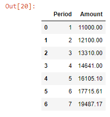
A common rule of thumb is what is known as the ‘Rule of 72’. It essentially states that at a given rate of 10% (which we used for this example); the principle should double after 7.2 years. If we look at our table below, we see that at period 7 (or year 7) that our principle has almost doubled. Thus, we can confirm that our calculation is accurate and can be trusted to make further inferences.

If we would like to store the results for a more traditional analysis, we can export it as an excel file using the code in the next code block. The screenshot of excel below that is exactly what it will store in the file. The ‘pd.to_excel’ method can also be used to specify a certain sheet to store the data so that you can update an existing file that you might already have.

				
					# now lets save it to an Excel Spreadsheet
results.to_excel('results.xlsx')
				
			
Pandas Excel Output of our Results Dataframe

Writing the Code: Using Python to Print a Bar Plot of the Compound Interest

Next up, we want to visualize the compound interest formula based on the parameters we chose. Below is a code snippet that will do just that. To make things look snazzy, I have decided to use the Seaborn library which works on top of matplotlib. A few of the settings I used included changing the color palette to something bright and more exciting (this is Compound Interest after all!) and the size of the plot.

By default, the plot printout can be quite small so changing it to 11 x 8 will give us something large enough that can be used in most presentations. Additionally, we can always cut the resolution down with Microsoft Paint, but we can’t do the reverse. Better to error on the side of caution. As you can tell, the final command to print the actual bar plot is a single line of code. This example is simple, but the output is professional in quality.

				
					# now lets plot it out
# We will be using Seaborn on top of MatPlotLib to make things
# look just right

sns.set(rc={'figure.figsize':(11,8)}) # make the graph readably large
sns.set_style('whitegrid') # change the background grid
sns.set_palette('Greens') # hange the color scheme

# now for the actual plot
sns.barplot(data = results, x ='Period', y = 'Amount').set_title('Compound Interest Plot')
				
			
Compound Interest Plot Using Seaborn

Conclusion

I hope this quick how-to guide on computing and outputting a graph for Compound Interest using python was helpful. With a few tweaks here and there, you will have a robust tool to create plots and tables either for your client or for yourself on the fly. Using Google Colab is an excellent choice for being able to update and code in various environments. In fact, if your code stores your plot or excel file to a web folder, it may be simple to update PowerPoints and other products on a whim. That said, if computing Compounding Interest using python isn’t your jam, then check out our web based Compound Interest Calculator. No coding required!

Facebook
Twitter
LinkedIn
Pinterest

Guy Money

As a formally trained Data Scientist I find excitement in writing about Personal Finance and how to view it through a lens filtered by data. I am excited about helping others build financial moats while at the same time helping to make the world a more livable and friendly place.

Leave a Reply

Your email address will not be published. Required fields are marked *

Scroll to top