Data Driven Money

Live. Work. Retire. Smart.

Simulate the 4 Percent Rule for Retirement with Python

Simulate Finance ObjectivesWhen it comes to planning for retirement, the 4% rule is considered the sacred rule for withdrawal. It essentially states, that given a diversified portfolio, a retiree can safely withdraw 4% from their retirement nest egg every year in retirement (a 30-year retirement is assumed).

In this article I will cover how to construct a simulation with the 4% rule for retirement as the premise in Python. Within the code you can adjust your own planning considerations and plot out your expected returns based on the random assignment of historical stock market returns over a defined period.

Note: I will be assuming a portfolio constructed of 100% Stocks (vs a 60% Stock and 40% Bond mix)… however this is easily modifiable.

You will need to have access to a Python environment either on your computer or in the cloud. If you would like more information on the 4% Rule so you can better follow the Python code then you can check out this article I wrote on the topic for a quick primer.

Below is what we will cover in this article.

Simulating the 4% Rule with Python

Getting Started

In this first block of Python code, the only thing being done is importing the appropriate libraries for data manipulation and eventual plotting. The random library will be used to randomly select a historical Stock Market return so it can be used to appropriately model a portfolio over the selected time periods.

				
					# Will need these to help with manipulating our data
import numpy as np
import pandas as pd
import random

# Will use these to plot everything out
import pandas as pd
import seaborn as sns
import matplotlib.pyplot as plt

# Use Pandas to reformat columns to be displayed with only
# two decimal points... like a currency
pd.options.display.float_format = '{:6.2f}'.format


Establishing Initial Investment Criteria

In the next block of code the initial parameters that define our notional portfolio are set. Only 4 variables are necessary to fully describe what we are looking to model.

  • InitialPrincipal – The starting retirement account balance.

  • YearsUntilRetirement – The number of years left that the retiree will be actively contributing to their retirement accounts.

  • YearlyContributionUntilRetirement – While not retired, the amount of money contributed on an annual basis to the retirement account being modelled.

  • YearsInRetirment – The number of years after retirement that the simulation should model.

Note: For this particular simulation, we will be compounding returns annually. For a more granular approach you can switch to monthly compounding but given the time frames we are looking at combined with the inherent volatility in returns I don’t believe its necessary.

				
					# Set initial variables to define our simulation
InitialPrincipal = 100000
YearsUntilRetirement = 20
YearlyContributionUntilRetirement = 5000
YearsInRetirement = 40


After the initial variables are set, those same variables are appended to a Pandas DataFrame called data. There are 2 cases that need to be considered.

  1. Case 1: The simulation is assuming the investor is not yet retired and that there are greater than 0 working years left. In this case, annual contributions will be expected to be non-zero.

  2. Case 2: The simulation is run assuming that the portfolio is already in ‘retirement mode.’ In this case, we don’t need to consider an annual contribution.

				
					# data generated from the simulation will be stored here
data = pd.DataFrame(columns=['Year',
                             'Principal',
                             'Contribution',
                             'Distribution',
                             'Rate'])

# Year 1 Data is appended. Note, they need to be set differently
# depending if there are 0 years until retirement or more than 0

if (YearsInRetirement > 0) :
  data = data.append({'Year': 1, 'Principal': InitialPrincipal,
                      'Contribution':YearlyContributionUntilRetirement,
                      'Distribution': 0,
                      'Rate': 0}, ignore_index = True)
  
if (YearsInRetirement == 0) :
  data = data.append({'Year': 1, 'Principal': (0.96*InitialPrincipal),
                      'Contribution': 0, 'Distribution': (0.04*InitialPrincipal),
                      'Rate': 0}, ignore_index = True)


Using Historical S&P 500 Returns for Pool of Future Returns

Using the dataset provided by Slickcharts in CSV form here we can import the Total Return by the S&P 500 from 1926 to 2021. By bootstrapping from this dataset, we can simulate a given year’s return in the future.

If the S&P is not a preferred benchmark for the portfolio that you are trying to model, then you can add in your own data here. For example, if you are looking to model a 60% Stock / 40% Bond Portfolio then you can just input the data here. Also, if you are looking to adjust for inflation then you can simply just subtract each year’s measured inflation (e.g. CPI) from the returns column.

				
					returns = pd.read_csv('sp500returns-since-1926.csv', header = None)
returns = returns.rename(columns ={0:'Year', 1:'Returns'})
returns.head()


Returns DataFrame Output

Creating a Function for Investment Returns: Pre-Retirement

In order to calculate and store the simulation data (e.g., each year’s returns on principal and withdrawal amounts) we will be executing the same few lines of code repeatedly. Thus, for this exercise I will create a function to handle everything with as little code as necessary.

But first let’s look at the components of what will constitute our new function. Essentially, two for loops will be used. The first loop will calculate the growth of the principal while the portfolio has active contributions (during working years). This code can be seen below.

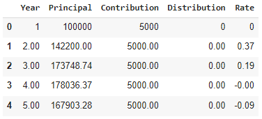
Last year’s interest is multiplied by a value found randomly in our random_return DataFrame and then the yearly contribution is added and stored as the current year’s principal. No withdrawal or distribution is subtracted since the portfolio hasn’t reached retirement mode yet.

				
					# Here we will iterate through the number of years until retirement
# adding the yearly contribution and compounding annually via a randomly
# selected value from our 'returns' DataFrame
for i in range(YearsUntilRetirement - 1):

  # calculate new year field
  NewYear = i+2

  # grab a random interest rate
  random_return = random.choice(returns['Returns']) /100

  # apply the random interest rate to last year's balance and add contribution
  NewPrincipal = data.loc[i]['Principal']*(1 + random_return)+YearlyContributionUntilRetirement
  
  data = data.append({'Year': NewYear, 'Principal': NewPrincipal,
                      'Contribution': YearlyContributionUntilRetirement,
                      'Distribution': 0,
                      'Rate': random_return}, ignore_index = True)


Creating a Function for Investment Returns: During Retirement

The next for loop iterates through each year after retirement and calculates that year’s withdrawal rate and associated interest from a random value in random_return. 0.96 is the factor used to decrement the principal since this excludes the 4% distribution (withdrawal) rate.

				
					# Now we will iterate through our years of retirement with another for loop
for i in range(YearsInRetirement):

  # calculate new year field
  NewYear = data.iloc[i+YearsUntilRetirement-1]['Year'] + 1
  
  # grab a random interest rate
  random_return = random.choice(returns['Returns']) /100

  # calculate the 4% distribution from last year's ending principal
  NewDistribution = data.loc[i+YearsUntilRetirement-1]['Principal']*(.04)

  # apply the random interest rate to 96% of last year's balance
  NewPrincipal = (.96)*data.loc[i+YearsUntilRetirement-1]['Principal']*(1 + random_return)
  
  data = data.append({'Year': NewYear, 'Principal': NewPrincipal,
                      'Contribution': 0,
                      'Distribution': NewDistribution,
                      'Rate': random_return}, ignore_index = True)


Below you can see the resulting DataFrame data. Notice the rate column… the returns for each year can vary widely just like the market. Afterall, these were actual market returns for the S&P 500 at some point in history!

				
					data.head()


Data DataFrame Output

Creating a Function for Investment Returns: Putting it All Together

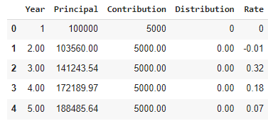
Below we actually create our function and name it retire4. By calling and running this function with the required arguments (the initial 4 variables we defined earlier) it will return a DataFrame with the same columns as above.

				
					def retire4(InitialPrincipal, YearsUntilRetirement, YearlyContributionUntilRetirement, YearsInRetirement):

      # data generated from the simulation will be stored here
      data = pd.DataFrame(columns=['Year',
                                   'Principal',
                                   'Contribution',
                                   'Distribution',
                                   'Rate'])
    
      # Year 1 Data is appended. Note, they need to be set differently
      # depending if there are 0 years until retirement or more than 0
    
      if (YearsInRetirement > 0) :
        data = data.append({'Year': 1, 'Principal': InitialPrincipal,
                            'Contribution':YearlyContributionUntilRetirement,
                            'Distribution': 0,
                            'Rate': 0}, ignore_index = True)
        
      if (YearsInRetirement == 0) :
        data = data.append({'Year': 1, 'Principal': (0.96*InitialPrincipal),
                            'Contribution': 0, 'Distribution': (0.04*InitialPrincipal),
                            'Rate': 0}, ignore_index = True)
        
      # Here we will iterate through the number of years until retirement
      # adding the yearly contribution and compounding annually via a randomly
      # selected value from our 'returns' DataFrame
      for i in range(YearsUntilRetirement - 1):
    
        # calculate new year field
        NewYear = i+2
    
        # grab a random interest rate
        random_return = random.choice(returns['Returns']) /100
    
        # apply the random interest rate to last year's balance and add contribution
        NewPrincipal = data.loc[i]['Principal']*(1 + random_return)+YearlyContributionUntilRetirement
        
        data = data.append({'Year': NewYear, 'Principal': NewPrincipal,
                            'Contribution': YearlyContributionUntilRetirement,
                            'Distribution': 0,
                            'Rate': random_return}, ignore_index = True)
       
        # Now we will iterate through our years of retirement with another for loop
      for i in range(YearsInRetirement):
    
        # calculate new year field
        NewYear = data.iloc[i+YearsUntilRetirement-1]['Year'] + 1
        
        # grab a random interest rate
        random_return = random.choice(returns['Returns']) /100
    
        # calculate the 4% distribution from last year's ending principal
        NewDistribution = data.loc[i+YearsUntilRetirement-1]['Principal']*(.04)
    
        # apply the random interest rate to 96% of last year's balance
        NewPrincipal = (.96)*data.loc[i+YearsUntilRetirement-1]['Principal']*(1 + random_return)
        
        data = data.append({'Year': NewYear, 'Principal': NewPrincipal,
                            'Contribution': 0,
                            'Distribution': NewDistribution,
                            'Rate': random_return}, ignore_index = True)
      return data


Below we will test our new function to see if it works as desired. We will put the variables defined earlier as arguments and store it in a DataFrame named data2. Subsequently, we’ll output the first 5 rows to see how it compares to our output above.

As you can see, it looks quite similar. The rate column has randomly assigned return values, so the numbers won’t match exactly but everything looks like the check out.

				
					data2 = retire4(InitialPrincipal, YearsUntilRetirement, YearlyContributionUntilRetirement, YearsInRetirement)
data2.head()


Data2 DataFrame Output

Plotting Our Results for a Single Result

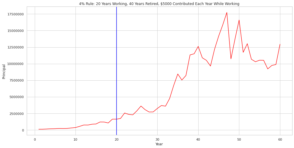
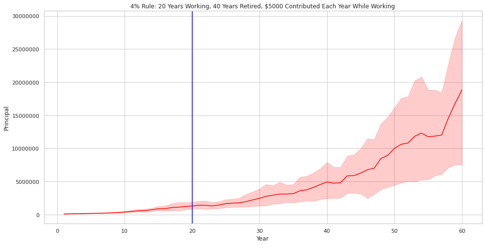
Now it’s time to see what a single trial of our simulation looks like when plotted out. Using MatPlotLib and Seaborn we can quickly plot out the results of data2.

I plotted a blue vertical line to denote the transition from working to retired. This also shows when contributions stop, and withdrawals start.

Given the long time period of the plot (60 years in this case), volatility seems to substantially increase during the later years, but this is just due to working with larger principals that have compounded for long periods.

By eventually plotting out large numbers of trials we should be able to smooth out the variability during later years of retirement.

				
					sns.set(rc={'figure.figsize':(16,8)}) # make the graph readably large
sns.set_style('whitegrid') # change the background grid
sns.set_palette('Greens') # hange the color scheme
plt.ticklabel_format(style='plain', axis = 'y') # prevent sci notation on y-axis

sns.lineplot(x="Year", y="Principal", data = data2, color = 'red').\
            set_title('4% Rule: ' + str(YearsUntilRetirement) +" Years Working, " + 
                      str(YearsInRetirement) + " Years Retired, $" +
                      str(YearlyContributionUntilRetirement)+" Contributed Each Year While Working")
            
# Add a vertical line to mark retirement
plt.axvline(x=YearsUntilRetirement, color= 'blue')


4% Rule 1Trial Simulation for Principal

Simulating Retirement Outcomes Across 10 Trials

Now let’s simulate the results for 10 trials. To do this I will create a new DataFrame called simulation and simply call our previously created retire4 function 10 times in a for loop.

				
					simulation = pd.DataFrame(columns=['Year',
                               'Principal',
                               'Contribution',
                               'Distribution',
                               'Rate'])

for i in range(10):
  simulation = simulation.append(retire4(InitialPrincipal,
                                         YearsUntilRetirement,
                                         YearlyContributionUntilRetirement,
                                         YearsInRetirement),
                                 ignore_index = True)


Using the describe() method available to us in simulation we can get some quick descriptive statistics to get an idea ahead of time of what our plot should show.

First, you can see that the count of Year is 600. This is just because we append 10 runs of 60 years. Next you can see the variability in Rate… there are 95 unique values in this field. It appears that our random function did a good job at allowing our simulation to utilize most of the 96 values available in returns.

				
					simulation.describe()


Simulation DataFrame Output

Plotting Retirement Outcomes Across 10 Trials

Now that we have generated the data, plotting out our 10-run simulation is simple. Seaborn will automatically plot a line for the mean and highlight the range of the Standard Deviation that bounds the mean line.

				
					sns.set(rc={'figure.figsize':(16,8)}) # make the graph readably large
sns.set_style('whitegrid') # change the background grid
sns.set_palette('bright') # hange the color scheme
plt.ticklabel_format(style='plain', axis = 'y') # prevent sci notation on y-axis

sns.lineplot(x="Year", y="Principal", data = simulation, color = 'red').\
            set_title('4% Rule: ' + str(YearsUntilRetirement) +" Years Working, " + 
                      str(YearsInRetirement) + " Years Retired, $" +
                      str(YearlyContributionUntilRetirement)+" Contributed Each Year While Working")
            
# Add a vertical line to mark retirement
plt.axvline(x=YearsUntilRetirement, color= 'blue')


4% Rule 10 Trial Simulation for Principal

As should be expected, the variability once again at the end of the 60-year period is significant. This should not be a cause for alarm. The large number of random outcomes possible is what creates this wide channel.

From this simulation it does appear that the 4% rule is a safe withdrawal rate. It does not look like that the principal is ever at risk of being depleted.

But what does the 4% withdrawal amount actually look like? Is it enough to live on? I’ll cover that next.

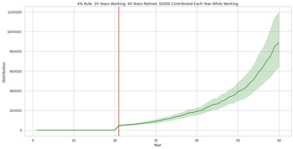
Plotting Annual Distributions at 4% for 10 Trials

Plotting out the annual distributions or withdrawals for the 10-run simulation only requires a variable change in the code below. I changed the colors as well to help highlight the different interpretation of the plot.

				
					sns.set(rc={'figure.figsize':(16,8)}) # make the graph readably large
sns.set_style('whitegrid') # change the background grid
sns.set_palette('bright') # hange the color scheme
plt.ticklabel_format(style='plain', axis = 'y') # prevent sci notation on y-axis

sns.lineplot(x="Year", y="Distribution", data = simulation, color = 'green').\
            set_title('4% Rule: ' + str(YearsUntilRetirement) +" Years Working, " + 
                      str(YearsInRetirement) + " Years Retired, $" +
                      str(YearlyContributionUntilRetirement)+" Contributed Each Year While Working")
            
# Add a vertical line to mark first year of distribution
plt.axvline(x=YearsUntilRetirement+1, color= 'red')


4% Rule 10 Trial Simulation for Withdrawals

As you can see above, the withdrawal rate does deviate from year to year but on average, it does generally go up. Keep in mind that this does not include the effects of inflation, however, the 4% Rule tackles this by assuming your portfolio grows enough each year to make up for this shortfall.

Simulating Retirement Outcomes Across 100 Trials

Now let’s see how running 100 trials changes things. Theoretically, our Standard Deviation depicted by the light red and green channels will narrow as we run more trials.

This narrowing doesn’t necessarily give us better information on how our portfolio will perform, but it will highlight the long-term uptrend of the Stock Market.

				
					simulation100 = pd.DataFrame(columns=['Year',
                               'Principal',
                               'Contribution',
                               'Distribution',
                               'Rate'])

for i in range(100):
  simulation100= simulation100.append(retire4(InitialPrincipal,
                                              YearsUntilRetirement,
                                              YearlyContributionUntilRetirement,
                                              YearsInRetirement),
                                     ignore_index = True)

# see the top few rows of simulation100
simulation100.head()


simulation100 DataFrame Output

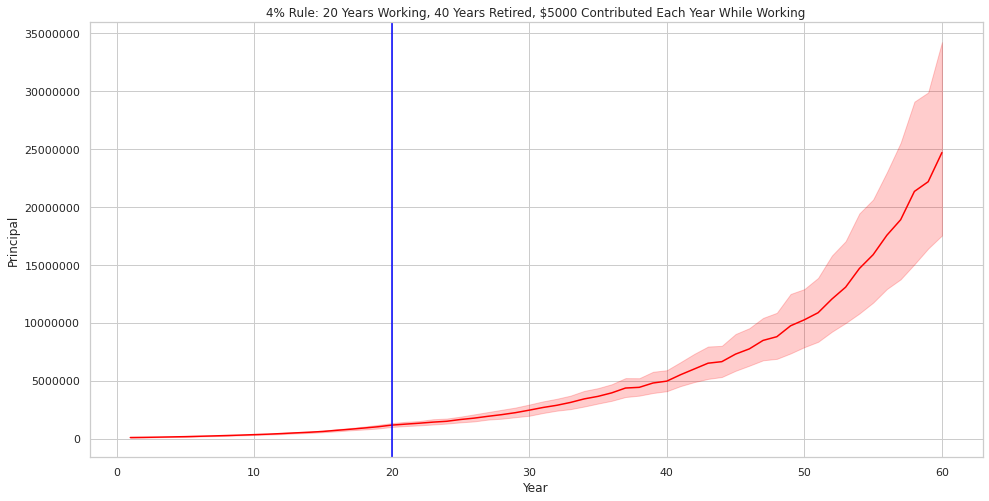
Plotting Retirement Outcomes Across 100 Trials

Below is the resulting plot of the principal. It frankly looks very similar to the 10 Trial plot with the exception that the channel is narrow, and the mean line is smoothed.

				
					sns.set(rc={'figure.figsize':(16,8)}) # make the graph readably large
sns.set_style('whitegrid') # change the background grid
sns.set_palette('bright') # hange the color scheme
plt.ticklabel_format(style='plain', axis = 'y') # prevent sci notation on y-axis

sns.lineplot(x="Year", y="Principal", data = simulation100, color = 'red', ci = 95).\
            set_title('4% Rule: ' + str(YearsUntilRetirement) +" Years Working, " + 
                      str(YearsInRetirement) + " Years Retired, $" +
                      str(YearlyContributionUntilRetirement)+" Contributed Each Year While Working")
            
# Add a vertical line to mark retirement
plt.axvline(x=YearsUntilRetirement, color= 'blue')


4% Rule 100 Trial Simulation for Principal

Plotting Annual Distributions at 4% for 100 Trials

Plotting out the withdrawals and distributions at 4% also results in a similiar smoother / narrower version of the 10 Trial simulation. The interpretation, once again, is that a 4% withdrawal rate seems to work just fine with a 100% Stock Portfolio over a long time horizon.

It should be also noted that this simulation assumes that the next 100 years in the Stock Market looks similar to the past 100 years. Smart folks out there would tell you that past performance doesn’t guarantee future results… buyer beware.

				
					sns.set(rc={'figure.figsize':(16,8)}) # make the graph readably large
sns.set_style('whitegrid') # change the background grid
sns.set_palette('bright') # hange the color scheme
plt.ticklabel_format(style='plain', axis = 'y') # prevent sci notation on y-axis

sns.lineplot(x="Year", y="Distribution", data = simulation100, color = 'green').\
            set_title('4% Rule: ' + str(YearsUntilRetirement) +" Years Working, " + 
                      str(YearsInRetirement) + " Years Retired, $" +
                      str(YearlyContributionUntilRetirement)+" Contributed Each Year While Working")
            
# Add a vertical line to mark first year of distribution
plt.axvline(x=YearsUntilRetirement+1, color= 'red')


4% Rule 100 Trial Simulation for Withdrawals

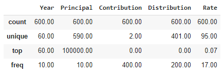
Calculating the 4% Rule Simulation Descriptive Statistics

Now that we’ve crunched the numbers and ran our simulation let’s see what the plots are telling us in a more specific fashion. Below you will find that on average you would be able to withdraw $46,820.95 during your first year of retirement. The standard deviation is significant at $36,396.

				
					# find the descriptive statistics for the amount of money you can safely withdraw (4%)
# during the first year in retirement
simulation100.loc[simulation100['Year'] == (YearsUntilRetirement+1)]['Distribution'].astype(int).describe()


Descriptive Stats 1

Below you can see that during the final year of retirement you can, on average, expect to withdraw $886,202.75. This may seem like a lot, but it would be helpful to consider inflation in this scenario.

After 60 years, if inflation compounds at 3% then $1.00 of spending power today would require $5.89 in the future. This means that $886,202.75 would have spending power of about $150,000 in today’s dollars.

				
					# find the descriptive statistics for the amount of money you can safely withdraw (4%)
# during the last year in retirement
simulation100.loc[simulation100['Year'] == (YearsUntilRetirement+YearsInRetirement)]['Distribution'].astype(int).describe()


Descriptive Stats 2

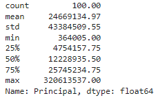
Below, you will see that on average you could expect to have $1.2 Million of principal during the first year of retirement.

				
					# find the descriptive statistics for the account balance
# during the first year in retirement
simulation100.loc[simulation100['Year'] == (YearsUntilRetirement+1)]['Principal'].astype(int).describe()


Descriptive Stats 3

And, at the end of retirement you could expect, on average, to have about $24.7 Million. That is the incredible power of compounding returns!

				
					# find the descriptive statistics for the account balance
# during the last year in retirement
simulation100.loc[simulation100['Year'] == (YearsUntilRetirement+YearsInRetirement)]['Principal'].astype(int).describe()


Descriptive Stats 4

Additional Considerations for Simulation

This is a great ‘first step’ simulation to get an idea if using the 4% rule for retirement withdrawals makes sense. Here are a few ideas and warnings on where to take the ideas presented in this article:

  • It would be easy to modify the function we created to run simulations for other percentages such as 3%, 3.5% or even 4.5% and 5%.

  • As mentioned previously, prior Stock Market performance does not predict future returns. Modifying the pool of returns for random assignment based on a more sophisticated outlook could substantially change the result of the simulation.

  • More trials does not necessarily mean more confidence in outcome. In fact, the more trials you run you will likely smooth out a few trials that could highlight problems with your investment approach. The right sequence of poor returns combined with withdrawals could be devastating and be missed if you just look at the scenario mean and standard deviation.

  • Inflation is generally considered ‘taken care of’ when using the 4% rule… thus, interpreting the final principal and withdrawal amounts need context. It does appear from our simulation that over the long term the spending power of a retiree may go up, however.

Final Thoughts

I hope you enjoyed this article! If you have any other thoughts about how to make the simulation better or ideas on how to better communicate the results be sure to throw them in the comments below!

Guy Money

As a formally trained Data Scientist I find excitement in writing about Personal Finance and how to view it through a lens filtered by data. I am excited about helping others build financial moats while at the same time helping to make the world a more livable and friendly place.

Leave a Reply

Your email address will not be published. Required fields are marked *

Scroll to top