Data Driven Money

Live. Work. Retire. Smart.

Hack Together a Debt Snowball Calculator With Python

Snowball method pay off debt. financial concept.The Debt Snowball is a repayment strategy that prioritizes paying back loans with the smallest balances first. This method is widely touted as being successful not for its mathematical superiority but buy its ability to take advantage of human psychology. The Debt Snowball Calculator can help identify the exact payment requirements… and outcome.

Dave Ramsey, the personal finance guru himself, advocates for the use of the Snowball Method (as opposed to the Debt Avalanche). But how does someone plan various scenarios with this payment strategy given the complexity and tediousness of the math involved?

With a few lines of Python code, you can quickly and seamlessly automate a repayment schedule built around the Snowball Method.

In this article I will show how to code your own Debt Snowball Calculator in Python. I will cover how to create your own snowball function and plot out relevant results using the Seaborn library to analyze whatever financial scenario you throw at it.

Navigating the Debt Snowball Calculator

Getting Started with Python

Before I get the ball rolling I should note that when making financial calculations it is always a good idea to have the ability to double check your work. For Debt Snowballs, I can think of no better tool to verify the validity of the code presented than comparing our results with the spreadsheet available from Vertex42.

To execute the code on this page you will need to use a Python Environment on your local machine. I highly recommend using Anaconda to help you navigate this, but there is also the ability to use a Python environment in the cloud.

Google provides a free Python cloud environment called Google Colab available here.

Furthermore, given the initial exploratory nature of this article, I do recommend using a Jupyter notebook (or Google Colab) so that code blocks can be executed, and results viewed in a manner where you can take notes.

Initial Requirements

The first code block below simply loads the required libraries for data manipulation. The pandas option set on the last line is only used to truncate float variables. There is no need to see anything past 2 decimal points considering we are working with dollars and cents.

				
					# import the python libraries needed for data manipulation
import pandas as pd
import numpy as np

# Use Pandas to reformat columns to be displayed with only
# two decimal points... like a currency
pd.options.display.float_format = '{:6.2f}'.format


Importing the Required Loan Information for a Debt Snowball

In order to compute the Debt Snowball payment schedule, we need to know the details of all of the loans. The 4 components of each loan that needs to be imported are:

  • The Name of the Creditor
  • The Current Balance of the Loan
  • The Interest Rate of the Loan
  • The Current Minimum Payment of the Loan

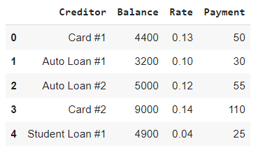
I have chosen to use a simple Excel file as a way to input this information for import into a pandas environment.

The format I used was a replica of the input cells required for our benchmark, the spreadsheet available from Vertex42 and can be seen below. You can very easily recreate this quickly for your own purposes.

Excel Output of Loan Information

The code below uses Pandas to import this spreadsheet directly from a local directory. If you are using Colab, simply drag and drop the excel file onto the file folder on the left side navigation pane.

				
					# import the loan information from an excel file and store in a DataFrame
# called 'loanInformation' then print it out to verify it imported properly
loanInformation = pd.read_excel('loan-information.xlsx')
loanInformation


Initial Output of Loan Information

Sorting the Loans by Balance

Since the Debt Snowball needs the loans to be sorted by balance we will go ahead and do that below. If we chose to instead sort by highest interest rate, then we would inadvertently be using the Avalanche Method.

				
					# The debt snowball requires that the loans be paid off by the smallest 
# balance first, thus for ease let's sort the DataFrame accordingly.
loanInformation = loanInformation.sort_values(axis = 0, by = 'Balance')
# clean up index
loanInformation = loanInformation.reset_index()
loanInformation = loanInformation.drop('index', axis =1)
# show the result
loanInformation


Initial Output of Loan Information Sorted

Establishing the Snowball

To start we need to establish our snowball amount. Usually, a debtor is asked to identify the total amount one can dedicate towards paying down debt. This includes the minimum required monthly amount and anything on top.

Theoretically, identifying the max that can be applied towards debt is an independent exercise from analyzing the debts themselves. In our code, this variable will be called maxPayment and should be set by the debtor after careful thought and consideration.

Thus, to calculate our Debt Snowball variable (which we will simply call snowball) we will need to add up the current minimum monthly payments (minRequired) and subtract the total from the overall amount the debtor has identified they can pay towards those debts.

				
					# Establish maxPayment variable. In our case we will use $500 as the maximum 
# amount.
maxPayment = 500

# Find the sum of all payments required per month
minRequired = loanInformation['Payment'].sum()

# Calculate the initial snowball. This will grow as debts are paid off.
snowball = maxPayment - minRequired

# Print out the values of our new variables
print('The Maximum Payment as Designated by the Debtor is: $', maxPayment)
print('The Minimum Amount that must be paid for all loans is: $', minRequired)
print('The Debt Snowball, or the amount extra being paid each month is: $', snowball)


Printed Output of Snowball Calculation

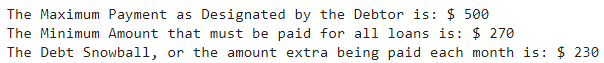
As can be seen above, if we add all the minimum payments together you get $270. Since the max we can pay each month is $500 the snowball will be $230. As we begin to pay off loans entirely, the snowball will start to grow and our ability to tackle the larger debts will increase.

Tracking Payoff Month

Now we need to add an additional column to keep track which month is which. The initial data will be denoted as Month ‘0’ and the value will increase until the loan is paid off completely.

				
					# Add a new column for Month and initialize it to 0
loanInformation['Month'] = 0
loanInformation


Output of Loan Information with Month Initialized

Preparing Tracking Variables for Our For Loop

Next, I will setup a for loop to test that our calculations come up with the right answer. It is always best to verify the methodology before you implement it after all.

Initializing the variables necessary for the loop comes first. numOfLoans is simply the number of creditors. This list is what will be looped through.

The variable workingSnowball is the amount of the snowball available to pay the next loan. This will include additional snowball if a loan gets paid off at some point or less snowball if a previously loan used some or all of it.

loanInformationMonth1, a DataFrame, will be used to store all the results for this test run of our calculations.

				
					# count the number of loans 
numOfLoans = len(loanInformation.index)

# create a working snowball variable to track additional portions of the 
# snowball that can be used during months when only part is used for a loan
workingSnowball = snowball

# create a new DataFrame with Month 1's Data
loanInformationMonth1 = pd.DataFrame(columns = ['Creditor',
                                                'Balance',
                                                'Rate',
                                                'Payment',
                                                'Month'])


The For Loop to Obtain One Month’s Payment Data

The actual loop is quite simple but there is one detail that does need to be addressed.

When a debtor pays the minimum amount on a loan, the balance only goes down a fraction of that. Each payment is comprised of the interest and principal portions. We will need to calculate these components.

The logic for each statement can be found in the comments below.

				
					# Let's Use a For Loop to Iterate through each loan
for i in range(numOfLoans):
  # if the Balance is > 0 then continue
  if(loanInformation.iloc[i]['Balance']> 0 ):
    # increment the month
    newMonth = loanInformation.loc[i]['Month'] + 1
    # Subtract the princpal only portion of the payment from the balance 
    interestPortion = loanInformation.iloc[i]['Balance'] * (1/12)*loanInformation.iloc[i]['Rate']
    principalPortion = loanInformation.iloc[i]['Payment'] - interestPortion
    # if some of the snow ball is left see how much can be used towards this loan
    if(workingSnowball > 0):
      # if the snowball is not bigger than the remaining balance...
      if(workingSnowball < (loanInformation.iloc[i]['Balance']-principalPortion)):
        # assign new princpal less the principal portion of the payment and snowball
        newPrincipal = loanInformation.iloc[i]['Balance']-principalPortion-workingSnowball
        # is now gone
        workingSnowball = 0
      # if the snowball is bigger than the remaining balance...
      else:
        newPrincipal = 0
        # figure out excess by taking inverse of potential overpayment
        workingSnowball = -1 * (loanInformation.iloc[i]['Balance']-principalPortion-workingSnowball)
    # If there is not snowball left then continue updating the balance
    else:
      # assign new princpal less the principal portion of the payment and snowball
        newPrincipal = loanInformation.iloc[i]['Balance']-principalPortion-workingSnowball
    # Append the new found data to our DataFrame
  loanInformationMonth1 = loanInformationMonth1.append({'Creditor': loanInformation.loc[i]['Creditor'],
                                                        'Balance': newPrincipal,
                                                        'Rate': loanInformation.loc[i]['Rate'],
                                                        'Payment': loanInformation.loc[i]['Payment'],
                                                        'Month': newMonth}, ignore_index= True)


Below is the output of the for loop found in the DataFrame loanInformationMonth1 .

Output of Loan Information after 1 Month For Loop

As we can see above Card #1 was paid down in the following manner:

The Principal Payment + The Snowball = $2.67 + $230.00 = $232.67

Thus, since the starting balance was $3,200, the new balance should be approximately $2966.32. This is nearly exactly what we were able to calculate using the code above.

But how do we apply this same methodology month in and month out?

Modifying the For Loop to Calculate all Payoff Data

Next, we need to figure out a way to iterate through each month while keeping tabs on our occassionally changing snowball.

My solution proposes that it would be beneficial to save all data collected along the way. To do this we will use a an expanded version of the same DataFrame to store additional results. This includes the partial interest and principal components for each payment and the total monthly amount applied for each loan.

We will need to approach the snowball method much in the same way as above except we will need move down the DataFrame for each month as we iterate through. We will keep a record of all transactions.

There will also need to be a while statement to determine if and when all balances have reached 0. This will prevent us getting caught into an infinite loop. Eventually we will move towards turning this into a function so this whole complicated looping business is invisible to the casual user.

The first code block once agains sets up a few tracking variables for the eventual looping.

				
					# create a new DataFrame that will contain all data for all months with initial 
# data copied over
loanInformationAll = loanInformation.reset_index()
# Add a few new fields for future analysis
loanInformationAll['Snowball'] = snowball
loanInformationAll['PaymentPrincipal'] = 0
loanInformationAll['PaymentInterest'] = 0

# Create a Complete Flag to let while loop know when all accounts are paid off
completeFlag = True


Next is the while loop. It will quit looping once the sum of all remaining balances are less than or equal to 0. The nested for loop is very similiar to the one previously used with a few additional complications necessary to track the proper index.

				
					# complete this loop until the accounts are complete
while completeFlag:  
  # This For loop will still iterate through i numOfLoans but when indexing it will
  # need to only access the numOfLoans... the most recent previous month calculated
  # instead if index i, it will now be the number of (last month calculated * numOfLoans + i)
  # which we wills store in a variable called indexTracker
  indexTracker = loanInformationAll.iloc[-1]['Month']*numOfLoans
  workingSnowball = snowball + loanInformationAll.loc[loanInformationAll['Balance'] <= 0].groupby('Creditor').median()['Payment'].sum()                                        
  for i in range(numOfLoans):
    # use an upgrade index tracker for the for loop
    forIndexTracker = indexTracker + i
    # if the Balance is > 0 then continue
    if(loanInformationAll.iloc[forIndexTracker]['Balance'] > 0 ):
      # increment the month
      newMonth = loanInformationAll.loc[forIndexTracker]['Month'] + 1
      # Subtract the princpal only portion of the payment from the balance 
      interestPortion = loanInformationAll.iloc[forIndexTracker]['Balance'] * (1/12)*loanInformationAll.iloc[forIndexTracker]['Rate']
      principalPortion = loanInformationAll.iloc[forIndexTracker]['Payment'] - interestPortion
      # if some of the snow ball is left see how much can be used towards this loan
      if(workingSnowball > 0):
        # if the snowball is not bigger than the remaining balance...
        if(workingSnowball < (loanInformationAll.iloc[forIndexTracker]['Balance']-principalPortion)):
          # assign new princpal less the principal portion of the payment and snowball
          newPrincipal = loanInformationAll.iloc[forIndexTracker]['Balance']-principalPortion-workingSnowball
          # is now gone
          workingSnowball = 0
        # if the snowball is bigger than the remaining balance...
        else:
          newPrincipal = 0
          # figure out excess by taking inverse of potential overpayment
          workingSnowball = -1 * (loanInformationAll.iloc[forIndexTracker]['Balance']-principalPortion-workingSnowball)
      # If there is not snowball left then continue updating the balance
      else:
        # assign new princpal less the principal portion of the payment and snowball
        newPrincipal = loanInformationAll.iloc[forIndexTracker]['Balance']-principalPortion-workingSnowball
    else:
      newPrincipal = 0
      principalPortion = 0
      interestPortion = 0
      newMonth = loanInformationAll.iloc[forIndexTracker]['Month']
    # Append the new found data to our DataFrame
    loanInformationAll = loanInformationAll.\
                    append({'Creditor': loanInformationAll.loc[forIndexTracker]['Creditor'],
                            'Balance': newPrincipal,
                            'Rate': loanInformationAll.loc[forIndexTracker]['Rate'],
                            'Payment': loanInformationAll.loc[forIndexTracker]['Payment'],
                            'PaymentPrincipal': principalPortion,
                            'PaymentInterest': interestPortion,
                            'Month': newMonth,
                            'Snowball': snowball + loanInformationAll.loc[loanInformationAll['Balance'] <= 0].groupby('Creditor').median()['Payment'].sum()  }, ignore_index= True)

    # If there are no more accounts with a balance then toggle our completeFlag
  if loanInformationAll.loc[loanInformationAll['Month'] == newMonth]['Balance'].sum() <= 0:
    completeFlag = False
    loanInformationAll = loanInformationAll.drop('index',axis=1)


Below are the results of running our new loop. The final 5 rows clearly show that all balances are at 0 and the final payment was made out to Card #2 with the exact principal and interest breakdowns shown.

The Vertex42 spreadsheet, our benchmark, also confirms that the final loan would be Card #2 during the 75th month. The loop works!

				
					loanInformationAll.tail(5)


Output of Loan Information All after 1 Full Loop

Creating a Python Function to Update Balances for All Months

Below, I take the successful looping code from above, strip out the comments and turn it into a Python function using the def statement. The only two inputs required to get the results we have achieved so far are:

  • The original loanInformation DataFrame from the excel spreadsheet in its original form (no sorting required)

  • The maxPayment, or the most the debtor can afford to pay each month including the minimum payments required by the lenders.

				
					# to create our new python function all we have to do is copy (mostly)
# the code we created above and annotate the input variables
# and output DataFrame

def snowballCalc(loanInformation, maxPayment):

  minRequired = loanInformation['Payment'].sum()
  snowball = maxPayment - minRequired

  loanInformationAll = loanInformation.sort_values(axis = 0, by = 'Balance').reset_index()
  loanInformationAll['Month'] = 0
  loanInformationAll['Snowball'] = snowball
  loanInformationAll['PaymentPrincipal'] = 0
  loanInformationAll['PaymentInterest'] = 0
  newMonth = 0
  completeFlag = True

  while completeFlag:  
    indexTracker = loanInformationAll.iloc[-1]['Month']*numOfLoans
    workingSnowball = snowball + loanInformationAll.loc[loanInformationAll['Balance'] <= 0].groupby('Creditor').median()['Payment'].sum()                                         
    for i in range(numOfLoans):
      forIndexTracker = indexTracker + i
      if(loanInformationAll.iloc[forIndexTracker]['Balance'] > 0 ):
        newMonth = loanInformationAll.loc[forIndexTracker]['Month'] + 1
        interestPortion = loanInformationAll.iloc[forIndexTracker]['Balance'] * (1/12)*loanInformationAll.iloc[forIndexTracker]['Rate']
        principalPortion = loanInformationAll.iloc[forIndexTracker]['Payment'] - interestPortion
        if(workingSnowball > 0):
          if(workingSnowball < (loanInformationAll.iloc[forIndexTracker]['Balance']-principalPortion)):
            newPrincipal = loanInformationAll.iloc[forIndexTracker]['Balance']-principalPortion-workingSnowball
            workingSnowball = 0
          else:
            newPrincipal = 0
            workingSnowball = -1 * (loanInformationAll.iloc[forIndexTracker]['Balance']-principalPortion-workingSnowball)
        else:
          newPrincipal = loanInformationAll.iloc[forIndexTracker]['Balance']-principalPortion-workingSnowball
      else:
        newPrincipal = 0
        principalPortion = 0
        interestPortion = 0
        newMonth = loanInformationAll.iloc[forIndexTracker]['Month']
      loanInformationAll = loanInformationAll.\
                    append({'Creditor': loanInformationAll.loc[forIndexTracker]['Creditor'],
                            'Balance': newPrincipal,
                            'Rate': loanInformationAll.loc[forIndexTracker]['Rate'],
                            'Payment': loanInformationAll.loc[forIndexTracker]['Payment'],
                            'PaymentPrincipal': principalPortion,
                            'PaymentInterest': interestPortion,
                            'Month': newMonth,
                            'Snowball': snowball + loanInformationAll.loc[loanInformationAll['Balance'] <= 0].groupby('Creditor').median()['Payment'].sum()  }, ignore_index= True)
    if loanInformationAll.loc[loanInformationAll['Month'] == newMonth]['Balance'].sum() <= 0:
      completeFlag = False
      loanInformationAll = loanInformationAll.drop('index',axis=1)
      return loanInformationAll


Below, we execute our new function and save the results into a DataFrame named df. The final 5 rows are displayed so we can ensure that they match our original results and those of our benchmark Excel spreadsheet.

				
					# now lets test our function with the raw data in the excel spreadsheet
# and setting our maxPayment to 500
df = snowballCalc(pd.read_excel('loan-information.xlsx'), 500)
df.tail(5)


Output of Loan Information All after 1 Full Loop

Plotting the Debt Snowball: Bar Chart of Interest Paid

Now that we have successfully calculated our results it is time to do something with them.

The first thing that might be interesting would be to visualize the amount of interest paid for each loan over the course repayment using the Snowball Method. To do this some data manipulation will need to occur. We will need to group all our results by Creditor and sum the interest components.

				
					# Find the total amount of interest paid for each creditor
totalPaymentInterest = df.groupby(by='Creditor').sum()[['PaymentInterest']]
# Make the index 'Creditor' an actual column for plotting
totalPaymentInterest.reset_index(inplace=True)
totalPaymentInterest


Output of Grouped Interest Components

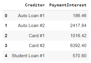
From there we will need to import 2 libraries to help us actually render the plot: matplotlib and seaborn. Both libraries are very well known and will help us present our data quickly. Below is the code and the Plot.

				
					# These libraries will be needed for our plotting efforts
import seaborn as sns
import matplotlib.pyplot as plt

# Set some options with Seaborn for aesthetics
sns.set(rc={'figure.figsize':(12,8)}) # make the graph readably large
sns.set_style('whitegrid') # change the background grid

# prevent sci notation on y-axis
plt.ticklabel_format(style='plain', axis = 'y')

# Construct our Interest Paid Comparison Plot
toal_interest_barplot = sns.barplot(x='Creditor',
                                    y='PaymentInterest',
                                    data=totalPaymentInterest,
                                    label="Interest Paid").\
                                    set_title("Barplot of Total Interest Paid",
                                              fontsize = '20')
plt.show()


Barplot of Total Interest Paid

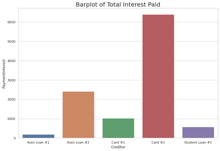
As you can see above, the prime offender when it comes to interest is Card #2. This is not the loan we attempted to pay off first with the snowball method.

In fact, Card #2 had the highest interest rate and largest balance… so we paid it off last. This clearly results in a situation where the debtor has paid off more interest than necessary. This highlights once again that when using the snowball, you are taking advantage of the psychological benefits of debt repayment and not necessarily mathematics.

Plotting the Debt Snowball: Timeline of Payoff

The following plot is an excellent way to visualize exactly how the snowball method functions. By plotting a line plot of each loan’s balance we will be able to see how the rate of change of repayment occurs.

				
					# Plot each debt as its own line over the course of each month
sns.lineplot(x="Month", y="Balance", hue = 'Creditor', data = df).\
                                    set_title("Linepolot of Individual Loan Balances Over Time",
                                              fontsize = '20')


Lineplot of Individual Loan Balances Over Time

The first loan paid off is Auto Loan #1 since it started with the smallest balance. Its rate of descent remains constant since it gets to use the snowball along with the minimum payment the entire time.

Moving to the left, the orange line shows how Card #1 declines over time. It descends only slightly until the first loan is paid off since its minimum payment barely covers any principal. Once the first loan is paid off it can use the snowball and the amount originally allocated to the monthly payment of Auto Loan #1. Once this occurs the balance drops much faster.

The same can be seen for each loan thereafter. As each loan is successively paid off, the next loan decreases in dramatic fashion.

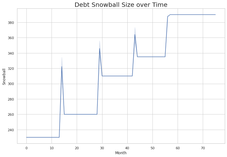
Plotting the Debt Snowball: Total Debt Over Time

The last chart I will show is not one that is necessarily interesting to someone who is repaying their debts. Rather, it shows that our function is working even when considering the nuances.

Consider that during a month that any of the loans are paid of there may be additional money available above and beyond what is owed for the last payment. The chart below shows that we are able to take care of this additional, albeit very small amount, correctly.

Notice the spike in debt snowball size during each of the months that a loan is fully paid off.

				
					# Plot each debt as its own line over the course of each month
sns.lineplot(x="Month", y="Snowball", data = df).\
                                    set_title("Debt Snowball Size over Time",
                                              fontsize = '20')


Debt Snowball Size Over Time

Debt Snowball vs the Debt Avalanche

Now that we have a quick way to generate the full repayment schedule utilizing a Debt Snowball methodology it would be beneficial to be able to compare this to its main competitor: The Avalanche Debt Repayment Method.

By automating our results for the Avalanche Method, we can quickly compare the practical differences of a mathematically minded approach versus a psychological one.

We can then know qualitatively the differences between the two approaches by being able to qualitatively establish various metrics such as:

  • How much longer does one approach take?
  • How much more interest is paid?
  • How long before the first loan is paid of?

Final Thoughts

In this article we were able to take a simple spreadsheet with loan information and ultimately create a reusable Python Function to implement the Debt Snowball strategy. From this function we were able to glean important facts about the repayment strategy.

More importantly, we created a tool that we can eventually use to help make informed decisions about specific situations. Although the Snowball Method is pretty cut and dry in its implementation, it can be difficult to communicate the implications for an individual who may be in the throes of debt.

I hope you enjoyed this article as much as I enjoyed writing it! Please feel free to drop any ideas or constructive criticisms in the comments below!

Guy Money

As a formally trained Data Scientist I find excitement in writing about Personal Finance and how to view it through a lens filtered by data. I am excited about helping others build financial moats while at the same time helping to make the world a more livable and friendly place.

Leave a Reply

Your email address will not be published. Required fields are marked *

Scroll to top