Data Driven Money

Live. Work. Retire. Smart.

How to Use Python to Code a Debt Avalanche Calculator

Avalanche SignThe Debt Avalanche, the lesser known cousin of the Debt Snowball, is a debt repayment strategy that prioritizes paying back those debts with the highest rates interest first. It is the most mathematically sound and efficient way to pay back a loan on a reoccurring basis.

Calculating what to pay 1 month from now using the Avalanche Method is very simple. But what about calculating those amounts for all months of repayment? What about calculating the risk / benefit metrics to compare against other methods?

Answering these questions is where the power of the Python language takes over.

In this article I will cover how to use Python to import a list of debts and calculate the amount that should be paid every month of repayment. Then I will show you how to tease out important information such as the total interest paid by loan and the number of months each loan spends in repayment.

Finally, I will help you develop a Python function that will make the process easily repeatable. It will allow you to quickly run an analysis on the Avalanche method so that an informed decision can be made by the debtor.

The Quick and Dirty Truth about the Debt Avalanche

Although this repayment method is the quickest method and backed up by simple math, it is often not preferred over other methods such as the Debt Snowball.

As mentioned in my article about How to Use Python to Code a Debt Snowball Calculator, the Debt Avalanche is not friendly to the average person’s Psychology. It focuses on paying off debts that have high interest rates. Paying off those debts first may take a long time before someone is able to witness any progress.

In comparison, the Debt Snowball prioritizes the debts with the smallest balances. The results appear to come quicker since it’s easier to get that ‘first win,’ when at least one of the debts is paid off. The appeal of the snowball is purely related to tricking a person via their emotions.

All that said, being able to fully compute the amount of interest paid for both methods is beneficial in that it gives us a quantitative measure of how they differ. By creating a Python function in this article, it will give us one of the tools necessary to moved down that path.

Below is a quick table of all the tasks we will complete in this article using Python.

Using Python to Make a Debt Avalanche Calculator

Getting Started with Python

To get started, you will need to make sure you have access to a standard Python environment. You can set one up using something like Anaconda or you can use one in the cloud like Google Colab. I use the latter. The dependencies are always updated and it’s free… not to mention that I can access my Notebooks on my phone or my desktop whenever I feel like using them.

If you decide to give Colab a shot, it is basically a Googlfied version of Jupyter Notebook.

Below you can see that we will be using very few libraries to start out. Most of the necessary functionality needed is just arithmetic… albeit a lot of it!

				
					# import libraries needed to manipulated data
import pandas as pd
import numpy as np

# ensure that float's only display a precision of 2
# making them appear 'currency-like'
pd.options.display.float_format = '{:6.2f}'.format


Importing and Preparing Our Loan Data

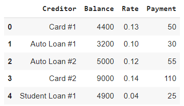
Next, we need to import our data. I used a simple Excel file to create a series of 5 notional loans. The following 4 bits of information for each loan is required to move further into the calculation stage:

  • Creditor – This identifies the loan uniquely.
  • Balance – This is the remaining balance of the loan.
  • Rate – This is the annualized interest rate of the loan.
  • Payment – This is the minimum mandatory payment necessary to keep the loan in good standing.

A screenshot of the Excel spreadsheet can be found below.

Excel Output of Loan Information

Once thet spreadsheet has been populated and saved in a place accessible to the Python environment, we can use Pandas’ read_excel method to import the data into a DataFrame. We will call our new DataFrame loanData. The full contents of loanData can be seen below.

				
					# load the loan data from an excel file and store
# into a DataFrame
loanData = pd.read_excel('loan-information.xlsx')
loanData


Initial Output of loanData

Sorting Our Loan Data by Interest Rate

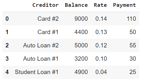
The Debt Avalanche pays off loans based off the highest interest rate. Going ahead and sorting loanData will allow us the ability to tackle the computation problem linearly. The new DataFrame can be seen below reindexed and in the proper order according to the field Rate.

				
					# The Debt Avalanche pays off debts with the highest
# 'Rate' first. Thus, we will sort it accordingly.
loanData = loanData.sort_values(by = 'Rate',
                                axis = 0,
                                ascending = False)

# Sorting loanData causes the index to be out of order
# so we need to fix it here.
loanData.reset_index(inplace = True)
loanData= loanData.drop('index', axis = 1)
loanData


Output of Sorted loanData

Defining the Avalanche

The Avalanche itself requires an amount that is above beyond the total sum of the minimum payments. The sum of the Payment field above is $270.

The maximum monthly payment would need to be greater than $270 to use the Avalanche method. For our scenario, we will set our maximum payment amount to $500 leaving us $230 additional each month to pay the debt according to our strategy.

The max payment would be set by the debtor after conducting a careful budgeting exercise. The code below sets maxPay and computes avalanche.

				
					# assing the max payment
maxPay = 500

# find the total sum of min payments
minReq = loanData['Payment'].sum()

# find the Avalanche, or excess amount 
avalanche = maxPay - minReq

# print the calculated values
print('The Max Payment is: $', maxPay)
print('The Total Min Required Payment is: $', minReq)
print('The Debt Avalanche amount is: $', avalanche)


Console Output for Avalanch

The Debt Avalanche Function: Requirements

Creating a function in Python is usually preferred when a task needs to be completed more than twice. Ideally, this new function we are going to create will be used much more than that. The logic of what we are about to undertake is very simple but may be difficult to conceptualize so I will break down the approach into bullet points.

  • I will first expand our DataFrame loanData to include other relevant metrics that may be useful when conducting a financial analysis. These will include the Month, the Current Value for Avalanche, and the Principal / Interest Breakdown of each payment for each loan during each month.

  • The function will take our initial loan DataFrame for input and once augmented with the fields in the bullet point above it will need to be updated with future calculations. These will be appended. We will calculate a local variable corresponding to each field in loanData that will need to be updated.

  • The ‘Avalanche Payment’ can vary from month to month. It will get larger as each loan is paid off. It can also be larger temporarily during months when a loan is paid off and the minimum monthly payment for that loan exceeds the remaining balance. I will track this through a variable called newAvalanche.

  • I will use a for loop to iterate through the loan balances each month. The length of the for loop is known since it is just the number of loans. What is not known, however, is the number of months it will take to pay off all the loans. Because of this, I will need to use a while loop which will continue to execute as long as the sum of all the values in Balance for the previous Month exceeds 0.

The Debt Avalanche Function: Prototype

Below is the initial creation of the additional metrics that will be tracked and the initialization of the local variables that will be used to append data to loanData.

				
					# We will want to track a few additional fields as we
# make our calculations for eventual analysis
loanData['Month'] = 0
loanData['Avalanche'] = avalanche
loanData['PaymentPrincipal'] = 0
loanData['PaymentInterest'] = 0

# Addtionally, we will want to have local variables that will
# change from month to month 
newBalance = 0
newPrincipalPortion = 0
newPaymentInterest = 0
newMonth = 0
newAvalanche = 0

# We will need to know the number of loans so we can iterate through them
numLoans = len(loanData)


Below is essentially the while loop with the nested for loop. The comments provided should help you identify the flow. At the end of the day, you should be able to confirm what I have determined already: this is tedious.

				
					# while the sum of remaining debt is > 0 from the previous month
while (loanData.loc[loanData['Month']==newMonth]['Balance'].sum() > 0):
  # we will use a for loop to iterate through each debt by month. Thus,
  # we will need to keep track of our indexes as multiples of our loans
  index = loanData.iloc[-1]['Month']*numLoans
  # our Avalanche will change if a loan is paid off at anypoint and needs to reset
  newAvalanche = avalanche + loanData.loc[loanData['Balance'] <=0].groupby('Creditor').median()['Payment'].sum()
  # iterate through debts for a single month
  for i in range(numLoans):
    # i and index will together will be the appropriate index
    newIndex = i + index
    # only conduct payment if loan is 0 or more
    if(loanData.iloc[newIndex]['Balance'] > 0):
      # set local variables
      newMonth = loanData.loc[newIndex]['Month'] + 1
      newPaymentInterest = loanData.iloc[newIndex]['Balance']*(1/12)*loanData.iloc[newIndex]['Rate']
      newPrincipalPortion = loanData.iloc[newIndex]['Payment'] - newPaymentInterest
      # newBalance will be determined by if their is any Avalanche to work with
      if(newAvalanche > 0):
        # Make sure newAvalanche isn't too big when paired with the min payment
        if(newAvalanche < (loanData.iloc[newIndex]['Balance']-newPrincipalPortion)):
          newBalance = loanData.iloc[newIndex]['Balance']- newPrincipalPortion - newAvalanche
          # for this month, the Avalanche has been depleted
          newAvalanche = 0
        # if our newAvalanche is larger than the remaining balance...
        else:
          newBalance = 0
          # retain extra newAvalanche balance for next debt by taking the inverse
          # of the overpayment (neg * neg is a positive!)
          newAvalanche = -1 *(loanData.iloc[newIndex]['Balance']-newPrincipalPortion-newAvalanche)
      # if no Avalanche left for this payment then calc balance normally.
      else:
        newBalance = loanData.iloc[newIndex]['Balance']-newPrincipalPortion
    else:
      newBalance = 0
      newPrincipalPortion = 0
      newPaymentInterest = 0
      newMonth = loanData.loc[newIndex]['Month']
    # Append all this new data to our DataFrame  
    loanData = loanData.append({'Creditor': loanData.loc[newIndex]['Creditor'],
                                'Balance': newBalance,
                                'Rate': loanData.loc[newIndex]['Rate'],
                                'Payment': loanData.loc[newIndex]['Payment'],
                                'PaymentPrincipal': newPrincipalPortion,
                                'PaymentInterest': newPaymentInterest,
                                'Month': newMonth,
                                'Avalanche': avalanche + loanData.loc[loanData['Balance'] <=0].\
                                            groupby('Creditor').median()['Payment'].sum()}, ignore_index= True)


With the looping finally complete, let’s take a look at the final few rows of loanData to see if it worked. Ideally, there would 0 (or slightly less than 0) left in the Balance column with differing values in the Month column denoting that each loan was paid off at a different time.

				
					loanData.tail(5)


loanData Preliminary

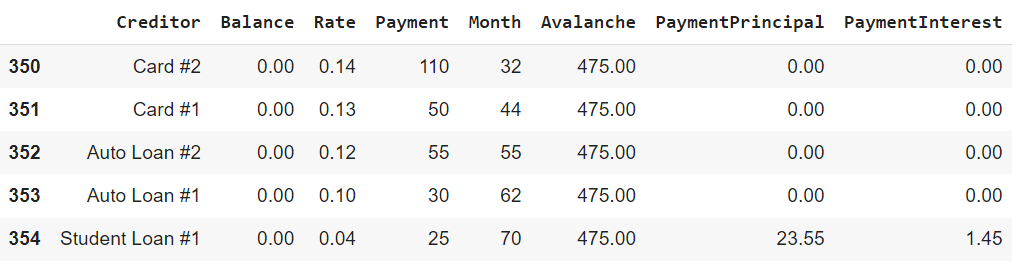
The output does seem to match expectations. It appears that using the Debt Avalanche method we were able to tackle all these loans in 70 months. In a separate article where I used these same debts with the Debt Snowball it took 75 months. By choosing this method we were able to save 5 months of repayment, although it may not have as been as psychologically stimulating.

The Debt Avalanche Function: The Final Product

Stripping out the comments (for the brevity of this article) and bounding our previous work in between a def and return statement we have our new Python function called avalancheCalc.

By passing the data from our Excel spreadsheet in along with our maximum monthly payment we will be returned the same DataFrame calculated above with the breakdown of each payment up until the avalanche has completely paid off all the loans.

				
					def avalancheCalc(loanData, maxPay):
      loanData = loanData.sort_values(by = 'Rate',
                                      axis = 0,
                                      ascending = False)
    
      loanData.reset_index(inplace = True)
      loanData= loanData.drop('index', axis = 1) 
      minReq = loanData['Payment'].sum()
      avalanche = maxPay - minReq
    
      loanData['Month'] = 0
      loanData['Avalanche'] = avalanche
      loanData['PaymentPrincipal'] = 0
      loanData['PaymentInterest'] = 0
    
      newBalance = 0
      newPrincipalPortion = 0
      newPaymentInterest = 0
      newMonth = 0
      newAvalanche = 0
    
      numLoans = len(loanData)
    
      while (loanData.loc[loanData['Month']==newMonth]['Balance'].sum() > 0):
        index = loanData.iloc[-1]['Month']*numLoans
        newAvalanche = avalanche + loanData.loc[loanData['Balance'] <=0].groupby('Creditor').median()['Payment'].sum()
        for i in range(numLoans):
          newIndex = i + index
          if(loanData.iloc[newIndex]['Balance'] > 0):
            newMonth = loanData.loc[newIndex]['Month'] + 1
            newPaymentInterest = loanData.iloc[newIndex]['Balance']*(1/12)*loanData.iloc[newIndex]['Rate']
            newPrincipalPortion = loanData.iloc[newIndex]['Payment'] - newPaymentInterest
            if(newAvalanche > 0):
              if(newAvalanche < (loanData.iloc[newIndex]['Balance']-newPrincipalPortion)):
                newBalance = loanData.iloc[newIndex]['Balance']- newPrincipalPortion - newAvalanche
                newAvalanche = 0
              else:
                newBalance = 0
                newAvalanche = -1 *(loanData.iloc[newIndex]['Balance']-newPrincipalPortion-newAvalanche)
            else:
              newBalance = loanData.iloc[newIndex]['Balance']-newPrincipalPortion
          else:
            newBalance = 0
            newPrincipalPortion = 0
            newPaymentInterest = 0
            newMonth = loanData.loc[newIndex]['Month']
          loanData = loanData.append({'Creditor': loanData.loc[newIndex]['Creditor'],
                                      'Balance': newBalance,
                                      'Rate': loanData.loc[newIndex]['Rate'],
                                      'Payment': loanData.loc[newIndex]['Payment'],
                                      'PaymentPrincipal': newPrincipalPortion,
                                      'PaymentInterest': newPaymentInterest,
                                      'Month': newMonth,
                                      'Avalanche': avalanche + loanData.loc[loanData['Balance'] <=0].\
                                                  groupby('Creditor').median()['Payment'].sum()}, ignore_index= True)
  return loanData


Testing the avalancheCalc Function

By executing the codeblock above, our new function should be loaded into the Python environment. Below we call on our function to pull in our raw data and conduct the same operations as before.

				
					# now lets test our function with the raw data in the excel spreadsheet
# and setting our maxPayment to 500
funcData = avalancheCalc(pd.read_excel('loan-information.xlsx'), 500)
funcData.tail(5)


loanData Confirmation

The last 5 rows of the DataFrame shown above matches what we were able to originally calculate confirming that our function was successful.

Plotting the Debt Avalanche: Bar Chart of Interest Paid

Understanding the amount of interest paid towards each loan over the course of the repayment strategy would be a good metric to visualize. To do this we will have to generate the grouped summary of the results.

The resulting table lists each loan and total interest paid over all periods.

				
					# Find the total amount of interest paid for each creditor
totalPaymentInterest = funcData.groupby(by='Creditor').sum()[['PaymentInterest']]
# Make the index 'Creditor' an actual column for plotting
totalPaymentInterest.reset_index(inplace=True)
totalPaymentInterest


loanDataTotal Interest

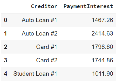
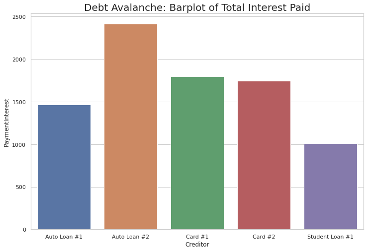
With totalPaymentInterest in hand we can now plot it out. A bar chart makes the most sense in this case given the structure of the data.

Below, I import seaborn and matplotlib to help with the plotting efforts. The plot shows that Auto Loan #2 was the biggest offender when it comes to interest payments.

Card #2 had the highest interest rate, however, it did not have the largest impact thanks to the Avalanche’s focus on minimizing debts with the highest rates.

				
					# These libraries will be needed for our plotting efforts
import seaborn as sns
import matplotlib.pyplot as plt

# Set some options with Seaborn for aesthetics
sns.set(rc={'figure.figsize':(12,8)}) # make the graph readably large
sns.set_style('whitegrid') # change the background grid

# prevent sci notation on y-axis
plt.ticklabel_format(style='plain', axis = 'y')

# Construct our Interest Paid Comparison Plot
toal_interest_barplot = sns.barplot(x='Creditor',
                                    y='PaymentInterest',
                                    data=totalPaymentInterest,
                                    label="Interest Paid").\
                                    set_title("Debt Avalanche: Barplot of Total Interest Paid",
                                              fontsize = '20')
plt.show()


Barplot of Total Interest Paid - Avalanche

Plotting the Debt Avalanche: Timeline of Payoff

Another interesting way to see how the Avalanche method actually works is to take a gander at the loan balances of each loan over the entire course of repayment.

When we do this, you will notice that the loan with the highest interest rate will descend the most rapidly at first until it hits 0. All other loans only descend slightly during this initial stage. After the first loan is paid off the next loan starts to rapidly decrease.

This process continues until all loans reach 0.

				
					# Plot each debt as its own line over the course of each month
sns.lineplot(x="Month", y="Balance", hue = 'Creditor', data = funcData).\
                                    set_title("Debt Avalanche: Linepolot of Individual Loan Balances Over Time",
                                              fontsize = '20')


Lineplot of Individual Loan Balances Over Time - Avalanche

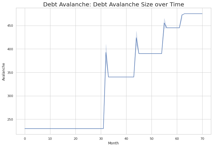
Plotting the Debt Avalanche: Total Debt Over Time

The final plot we will consider is the size of the Avalanche over time. It is useful in that it shows that we have considered some of the minor details. Below you will see that there is a sharp spike during the month that each loan is paid off. This occurs because, sometimes, during the month a loan is paid off the minimum monthly payment is more than the remaining balance.

The chart shows that we correctly identify this extra amount and apply it to our avalanche to be use for the next loan. This also can be seen in the previous chart when you see that some of the loans have a ’rounded’ corner (some have sharp ones).

				
					# Plot each debt as its own line over the course of each month
sns.lineplot(x="Month", y="Avalanche", data = funcData).\
                                    set_title("Debt Avalanche: Debt Avalanche Size over Time",
                                              fontsize = '20')


Avalanche Size Over Time

Final Thoughts

The Debt Avalanche is the fastest mathematical way to pay off a series of debts when you are trying to apply a small additional lump sum periodically during repayment.

Whether or not this methodology will lead to an average person paying off their debt quicker is up for interpretation. It may be too ’emotionally difficult’ to slog away at a high interest rate debt if there isn’t a feeling of ‘making progress.’ This ‘feeling’ can be engineered through less efficient methodologies such as the Debt Snowball.

Using our new function, however, we now have a tool to quantify what an optimal scenario looks like. Comparing the resulting metrics is a great way to get an idea of what exactly is lost in terms of repayment timeframe when another course of action is selected.

I hope you enjoyed this article… I certainly enjoyed writing it! If you have any comments about this article, both positive and constructive, feel free to throw them down below!

Guy Money

As a formally trained Data Scientist I find excitement in writing about Personal Finance and how to view it through a lens filtered by data. I am excited about helping others build financial moats while at the same time helping to make the world a more livable and friendly place.

Leave a Reply

Your email address will not be published. Required fields are marked *

Scroll to top